This was my first participation in a mathematical modeling competition. I ultimately won a second prize across the entire school. Award link: https://mp.weixin.qq.com/s/w1W8XwT2oHP4LlE9SSGCBw — this achievement was greatly encouraging, and I am now preparing to participate in the 2020 national competition.
The original title was “A Metro Route Planning Model Based on Multi-Traveling Salesman Problem and Its New Conceptions.” The “New Conceptions” part was completed by my teammates, so this blog post primarily describes my own thinking and problem-solving process, shared for learning and exchange.
Contents
- 1. Introduction
- 2. Preliminary Knowledge
- 3. Problem Analysis and Solution Approach
- 4. Model Construction and Solution
- 5. Model Evaluation and Summary
1. Introduction
1.1 Background
Student P plans to conduct a field survey of multiple transfer stations on the Guangzhou Metro. The survey includes recording the platform screen door numbers at each station and the relative positions of elevators and screen doors when switching between different lines. Since such information is not available on public platforms, it can only be obtained through personal visits to each transfer station.
The survey is subject to the following constraints:
- Flexible choice of start and end points: Both the departure and return locations can be chosen among Zhongda Station or Lujiang Station.
- Exclusion of specific lines: No investigation of transfer stations related to Line 9, Line 14, Line 21, or Line 13.
- APM line does not require separate investigation: The transfer and exit patterns of the APM line within metro stations are similar to ordinary lines, so it is not included in the survey scope.
- Exit and observation required at each station: Student P must exit the station to observe after arriving at each transfer station, then re-enter.
- Second passage through the same station does not require exiting: If a transfer station is visited twice, the second passage does not require exiting and may be passed through directly.
1.2 Problem Statement
Problem 1: How to select a survey route such that the total time to complete the survey of all 27 transfer stations is minimized, requiring departure from and return to the same station among Zhongda or Lujiang (single-day scheme).
Problem 2: Student P finds it physically unbearable to complete the entire survey within a single day, and plans to distribute the survey over 5 days. Each day starts from the starting point, completes that day’s survey, and returns to the end point. How to plan the daily routes so that the total time over 5 days is minimized.
Problem 3: Under the premise that the route plan from Problem 2 is determined, Student P’s uncle and aunt work at various transfer stations along Guangzhou Metro Line 8 every day, with workplaces chosen randomly and working hours covering the entire day. Calculate the expected total number of encounters between Student P and them individually, as well as the expected total number and variance of encounter counts.
2. Preliminary Knowledge
This chapter introduces the mathematical principles directly referenced in subsequent sections, primarily covering graph theory foundations, shortest path algorithms, combinatorial optimization, and probability theory. These topics have been systematically addressed in undergraduate discrete mathematics and probability courses; this chapter provides only concept definitions and result citations, omitting rigorous proofs.
2.1 Graph Theory Fundamentals
(1) Definition of a Weighted Undirected Graph
A graph $G(V, E, W)$ consists of three components: a vertex set $V = {v_1, v_2, \ldots, v_n}$, an edge set $E \subseteq V \times V$, and a weight function $W: E \rightarrow \mathbb{R}^+$. If for any vertex pair $(v_i, v_j) \in E$ we also have $(v_j, v_i) \in E$, and the weights satisfy $W(v_i, v_j) = W(v_j, v_i)$, then $G$ is called a weighted undirected graph.
After modeling, the metro network exactly constitutes a weighted undirected graph: transfer stations serve as vertices, metro line segments between stations serve as edges, and metro running times serve as edge weights.
(2) Adjacency Matrix and Reachability
Given a graph $G$ with $n$ vertices, the adjacency matrix $A$ is defined as an $n \times n$ matrix where:
$$A_{ij} = \begin{cases} W(v_i, v_j), & \text{if } (v_i, v_j) \in E \ 0, & \text{if } i = j \ \infty, & \text{otherwise} \end{cases}$$
The adjacency matrix describes the direct connectivity and weights between vertices. For non-adjacent vertex pairs, the corresponding matrix entry is infinity, indicating that direct access is impossible.
(3) Shortest Path Problem
The shortest path problem requires finding a path from a specified source to a destination such that the sum of all edge weights along the path is minimized. In a weighted undirected graph, there exist multiple classical algorithms for this problem, applicable to different scenarios.
2.2 Best Hamiltonian Cycle and Best Salesman Route
(1) Basic Definitions and Distinctions
Best Hamiltonian Cycle: Departing from a vertex, visiting all vertices in the graph exactly once, and returning to the starting point, forming a Hamiltonian circuit that minimizes the total edge weight.
Best Salesman Route: Departing from a vertex, visiting all vertices in the graph at least once, and returning to the starting point, minimizing the total edge weight. The difference between the two lies in the required number of vertex visits.
(2) Triangle Inequality and Complete Graph Transformation Conditions
Not all graphs contain a Hamiltonian cycle. Graph theory states that a Hamiltonian cycle necessarily exists if and only if the graph is complete (every pair of vertices is connected by an edge).
However, the Best Salesman Route problem does not require the graph to be complete. During solving, an incomplete graph can be transformed into a complete graph by an algorithm. If the weights of the newly added edges satisfy the triangle inequality:
$$W_{ik} \leq W_{ij} + W_{jk}$$
then the weight of the best Hamiltonian cycle obtained in this complete graph equals the weight of the best salesman route in the original incomplete graph. This transformation provides the foundation for subsequent solution methods.
2.3 Floyd Algorithm
(1) Algorithm Principles
The Floyd algorithm (also known as the Floyd-Warshall algorithm) is used to compute shortest paths between all pairs of vertices in a graph. Its core idea is dynamic programming.
Let $d^{(k)}_{ij}$ denote the shortest path from vertex $v_i$ to vertex $v_j$, where the intermediate vertices along the path have indices no greater than $k$. The recurrence relation is:
$$\min_{k} d_{ij}^{(k)} = \min\left(d_{ij}^{(k-1)}, d_{ik}^{(k-1)} + d_{kj}^{(k-1)}\right)$$
Initially, $d^{(0)}_{ij}$ equals the weight value in the adjacency matrix. By sequentially introducing vertices $1, 2, \ldots, n$ as intermediate points, the shortest path matrix is progressively updated until the shortest paths between all vertex pairs are obtained.
(2) Application in Complete Graph Transformation
The direct application of the Floyd algorithm is to find shortest paths, but in this problem it serves another clever purpose: using its results to complete an incomplete graph.
By taking the original graph’s adjacency matrix as input and computing the shortest path lengths between all pairs of vertices, and then adding these lengths as new edge weights to the graph, the incomplete graph $G$ can be transformed into a complete graph $G’$.
Since shortest paths themselves necessarily satisfy the triangle inequality $W_{ik} \leq W_{ij} + W_{jk}$, the complete graph $G’$ satisfies the prerequisite that the best Hamiltonian cycle and the best salesman route are equivalent. This step is a critical transition in the entire solution process.
2.4 Two-Edge Sequential Correction Algorithm (2-opt)
(1) Algorithm Principles
2-opt is a local search algorithm for solving the best Hamiltonian cycle. Given an initial circuit, if two non-adjacent edges $(v_i, v_{i+1})$ and $(v_j, v_{j+1})$ ($i < j$ and the two pairs of edges are non-adjacent) satisfy:
$$W_{i,j} + W_{i+1,j+1} < W_{i,i+1} + W_{j,j+1}$$
then replacing these two edges with $(v_i, v_j)$ and $(v_{i+1}, v_{j+1})$ can reduce the total circuit weight. After replacement, the node visit order in the circuit changes, which is vividly described as a “flip.”
(2) Iterative Process and Convergence Condition
The algorithm’s iterative steps are as follows:
- Arbitrarily provide a Hamiltonian circuit as the initial solution.
- Traverse all edge pairs $(i, j)$ that satisfy the condition and check whether the above inequality holds.
- If it holds, execute the replacement to obtain a better circuit.
- Repeat Steps 2–3 until, after traversing the entire graph, there are no replaceable edge pairs remaining.
Since each replacement strictly reduces the total weight and the weight has a finite lower bound, the algorithm must converge after a finite number of iterations, yielding a locally optimal solution — the best Hamiltonian cycle under the 2-opt criterion.
2.5 Minimum Spanning Tree and Prim Algorithm
(1) Minimum Spanning Tree Definition
Given a connected graph $G(V, E, W)$, a spanning tree $T$ is a subgraph of $G$ containing all $|V|$ vertices and $|V|-1$ edges with no cycles. The Minimum Spanning Tree (MST) is the spanning tree among all spanning trees with the smallest sum of edge weights.
The minimum spanning tree has two key properties: (1) it contains all vertices; (2) the sum of edge weights is minimal. These properties make it a powerful tool for network partitioning problems.
(2) Prim Algorithm Steps
The Prim algorithm is a classical algorithm for constructing a minimum spanning tree, adopting a greedy strategy. The steps are as follows:
- Arbitrarily select a starting vertex and add it to the tree.
- Repeat the following steps until all vertices have been added:
- Among all edges connecting vertices already in the tree to vertices not yet in the tree, select the one with the smallest weight.
- Add that edge and its unadded endpoint to the spanning tree.
- The result is a spanning tree containing all vertices, exactly $n-1$ edges, with the minimal total weight.
2.6 Fundamentals of Probability and Expectation
(1) Expectation of a Discrete Random Variable
Let a discrete random variable $X$ take values $x_1, x_2, \ldots, x_n$ with corresponding probabilities $p_1, p_2, \ldots, p_n$. Then the mathematical expectation of $X$ is:
$$E(X) = \sum_{k=1}^{n} x_k \cdot p_k$$
Expectation describes the average value of a random variable over repeated trials.
(2) Definition and Calculation of Variance
Variance measures the degree to which a random variable’s value deviates from its expectation, defined as:
$$\text{Var}(X) = E\left[(X - E(X))^2\right] = E(X^2) - [E(X)]^2$$
For a discrete random variable:
$$\text{Var}(X) = \sum_{k=1}^{n} (x_k - E(X))^2 \cdot p_k$$
3. Problem Analysis and Solution Approach
3.1 Data Source
All metro running time data between transfer stations in this paper are sourced from the Guangzhou Metro official website (http://www.gzmtr.com/). The raw data contains round-trip running times between adjacent stations. In this paper, the arithmetic mean of round-trip times is taken as each edge weight for modeling.
3.2 Model Assumptions
(1) It is assumed that Student P does not spend time when transferring at metro transfer stations (non-survey time).
(2) It is assumed that the time spent traveling in both directions between any two transfer stations is the same (and in practice the actual time spent is also roughly the same).
(3) Metro operation is in an ideal state, without delays or breakdowns or other force majeure factors.
3.3 Symbol Definitions
| Symbol | Meaning | Symbol | Meaning | |
|---|---|---|---|---|
| $t_1$ | Total time of metro running on routes | $W_{ij}$ | Weight between any two stations | |
| $t_2$ | Total time of surveying all transfer stations | $G$ | Graph | |
| $t$ | Total time Student P spends on routes | $G_i$ | Subgraph | |
| $t_i$ | Total time spent on any subgraph route | $E_i$ | Expected number of encounters with uncle/aunt on day $i$ | |
| $t_{1i}$ | Total time of metro running on any subgraph route | $P_j$ | Probability that uncle/aunt works at station $j$ | |
| $t_{2i}$ | Total time of surveying transfer stations on any subgraph | $Q_{ij}$ | Weight of encounter count at station $j$ on day $i$ | |
| $V$ | Set of all vertices | $T$ | Total time spent on all subgraph routes | |
| $E$ | Set of all edges |
3.4 Solution Principles and Methods
Problem 1: The best Hamiltonian cycle is equivalent to the shortest Hamiltonian circuit, corresponding to the method of using the Floyd algorithm to complete the graph and combining with 2-opt iterative solving.
Problem 2: The multi-traveling salesman route is decomposed into regional partitioning and sub-circuit optimization, corresponding to the method of using the Prim algorithm to generate a minimum spanning tree and, after partitioning regions, independently solving the best H circuit for each region.
Problem 3: The encounter count is a weighted discrete random variable, corresponding to the method of establishing a weight matrix $Q_{ij}$ and calculating the expectation $E_i = \sum_j P_j \cdot Q_{ij}$ and its variance.
4. Model Construction and Solution
4.1 Problem 1: Optimal Single-Day Survey Route
4.1.1 Problem Transformation
The total time $t$ consists of two parts:
$$t = t_1 + t_2$$
where $t_2$ is the sum of survey times at all stations, which can be directly accumulated after obtaining the actual survey time at each station and is a fixed value. $t_1$ is the total time Student P spends on metro routes, which depends on the chosen route and is the objective to be minimized.
Therefore, minimizing $t$ is equivalent to minimizing the metro running time $t_1$.
This problem corresponds to the Best Salesman Route Problem in graph theory: departing from a starting point, visiting all vertices at least once, and returning to the endpoint, minimizing the total edge weight. The difference from the classic Hamiltonian cycle problem is that each vertex need only be visited at least once, rather than exactly once.
4.1.2 Graph Simplification and Weight Definition
The Guangzhou Metro network is abstracted as a weighted undirected graph $G(V, E, W)$:
- Vertex set $V$: The 27 transfer stations requiring survey. Station numbers and corresponding names are listed in the table below:
| ID | Station Name | Survey Time (min) | ID | Station Name | Survey Time (min) | |
|---|---|---|---|---|---|---|
| 1 | Zhongda | — | 15 | Chebei South | 6 | |
| 2 | Guangzhou Railway Station | 8 | 16 | Xilao | 6 | |
| 3 | Yantang | 6 | 17 | Shayuan | 6 | |
| 4 | Tianhe Coach Station | 8 | 18 | Changgang | 6 | |
| 5 | Guangzhou East Station | 10 | 19 | Kecun | 8 | |
| 6 | Ouzhuang | 8 | 20 | Wanshengwei | 8 | |
| 7 | Gongyuanqian | 8 | 21 | Nanzhou | 6 | |
| 8 | Dongshankou | 8 | 22 | Lihua | 8 | |
| 9 | Yangji | 8 | 23 | University Town South | 6 | |
| 10 | Tiyu West Road | 15 | 24 | Shibi | 6 | |
| 11 | Tanwei | 6 | 25 | Hanxi Changlong | 6 | |
| 12 | Huangsha | 6 | 26 | Guangzhou South Station | 8 | |
| 13 | Haizhu Square | 8 | 27 | Jiahe Wangang | 6 | |
| 14 | Zhujiang New Town | 10 | — | — | — |
- Edge set $E$: The metro line segments between adjacent transfer stations. If two stations can be reached by a one-stop direct ride, there is one edge connecting the two vertices.
- Weight $W$: The time consumed by metro running between stations. Specifically, let the metro running time between two adjacent stations be $t$ (i.e., the edge weight), then $W_{ij} = t$. If two stations cannot be reached by a one-stop direct ride (i.e., no direct edge), then $W_{ij} = \infty$.
Since the original metro network does not have direct edges between any pair of vertices, the original graph $G(V, E, W)$ is an incomplete graph, and the best Hamiltonian cycle cannot be directly solved on it.
4.1.3 Floyd Algorithm for Complete Graph Completion
The Floyd algorithm (Floyd-Warshall algorithm) is used to compute shortest paths between all pairs of vertices in a graph, representing a classic application of dynamic programming.
Its core recurrence relation is: sequentially introducing vertex $k$ as an intermediate point, judging whether the path from vertex $i$ to vertex $j$ via $k$ is shorter than the currently known shortest path, and updating the shortest path length if so. The mathematical expression is:
$$\min_{k} d_{ij}^{(k)} = \min\left(d_{ij}^{(k-1)}, d_{ik}^{(k-1)} + d_{kj}^{(k-1)}\right)$$
Taking the original graph’s adjacency matrix as input and executing the Floyd algorithm yields the shortest path lengths between all pairs of vertices. Using these lengths as new edge weights and adding them to the graph transforms the incomplete graph $G$ into a complete graph $G’$.
Since shortest paths necessarily satisfy the triangle inequality $W_{ik} \leq W_{ij} + W_{jk}$, the weight of the best Hamiltonian cycle obtained in the complete graph $G’$ equals the minimal weight of the best salesman route in the original incomplete graph $G$. This step is a critical transition in the entire solution process.
The following is the MATLAB implementation of the Floyd algorithm:
function [path,road]=floyd(a)
    n=size(a,1);
    path=a;
    for i = 1:n
        for j = 1:n
            road(i,j) = j;
        end
    end

    for k=1:n
        for i=1:n
            for j=1:n
                if path(i,j)>path(i,k)+path(k,j)
                    path(i,j)=path(i,k)+path(k,j);
                    road(i,j)=road(i,k);
                end
            end
        end
    end
4.1.4 Best Hamiltonian Cycle Solving
On the complete graph $G’$, the Two-Edge Sequential Correction Algorithm (2-opt) is adopted to progressively optimize the initial circuit.
Given a Hamiltonian circuit, traverse any two non-adjacent edges $(v_i, v_{i+1})$ and $(v_j, v_{j+1})$ ($i < j$ and the two pairs of edges are non-adjacent). If satisfied:
$$W_{i,j} + W_{i+1,j+1} < W_{i,i+1} + W_{j,j+1}$$
then replace the original two edges with $(v_i, v_j)$ and $(v_{i+1}, v_{j+1})$, reducing the total circuit weight. Each completed replacement is called one “2-opt flip.” Repeatedly traverse and replace until, after traversing the entire graph, there are no improvable edge pairs; the algorithm converges, yielding a locally optimal Hamiltonian circuit — the sought best H cycle.
Repeatedly traverse and replace until, after traversing the entire graph, there are no improvable edge pairs; the algorithm converges, yielding a locally optimal Hamiltonian circuit — the sought best H cycle.
The following is the MATLAB implementation of the 2-opt algorithm:
function [b,s] = h(e)
    n=size(e);
    for i=2:n-2
        for j = i+1:n-2
            if e(i,j)+e(i+1,j+1)<e(i,i+1)+e(j,j+1)
                a=horzcat(e(:,1:i),e(:,j:-1:i+1),e(:,j+1:n));
                b=vertcat(a(1:i,:),a(j:-1:i+1,:),a(j+1:n,:));
                e=b;
            end
        end
    end
    s=0;
    for i=2:n-2
        s=s+e(i,i+1);
    end
4.1.5 Comparison of Two Schemes
The following is the complete MATLAB program code for solving Problem 1:
clc
clear
%Open the matrix with Zhongda as the start/end point to obtain Solution 1 for Problem 1
%Open the matrix with Lujiang as the start/end point to obtain Solution 2 for Problem 1
%Survey time at each station
t=[0 6 8 6 8 10 8 8 8 8 15 6 6 8 10 6 6 6 6 8 8 6 8 6 6 6 8];
%Define the adjacency matrix for Zhongda boarding/alighting station
a=[0 inf inf inf	inf	inf	inf	inf	inf	inf	inf	inf	inf	inf	inf	inf	inf	6	7	inf	inf	inf	inf	inf	inf	inf	inf;
0	0	inf	inf	inf	9	8	inf	inf	inf	12	inf	inf	inf	inf	inf	inf	inf	inf	inf	inf	inf	inf	inf	inf	inf	18;
0	0	0	6	4	12	inf	inf	inf	inf	inf	inf	inf	inf	inf	inf	inf	inf	inf	inf	inf	inf	inf	inf	inf	inf	18;
0	0	0	0	inf	inf	inf	inf	inf	14	inf	inf	inf	inf	inf	inf	inf	inf	inf	inf	inf	inf	inf	inf	inf	inf	inf;
0	0	0	0	0	inf	inf	inf	inf	6	inf	inf	inf	inf	inf	inf	inf	inf	inf	inf	inf	inf	inf	inf	inf	inf	inf;
0	0	0	0	0	0	inf	5	7	inf	inf	inf	inf	inf	inf	inf	inf	inf	inf	inf	inf	inf	inf	inf	inf	inf	inf;
0	0	0	0	0	0	0	9	inf	inf	inf	10	4	inf	inf	inf	inf	inf	inf	inf	inf	inf	inf	inf	inf	inf	inf;
0	0	0	0	0	0	0	0	4	inf	inf	inf	11	inf	inf	inf	inf	inf	inf	inf	inf	inf	inf	inf	inf	inf	inf;
0	0	0	0	0	0	0	0	0	4	inf	inf	inf	6	inf	inf	inf	inf	inf	inf	inf	inf	inf	inf	inf	inf	inf;
0	0	0	0	0	0	0	0	0	0	inf	inf	inf	4	inf	inf	inf	inf	inf	inf	inf	inf	inf	inf	inf	inf	inf;
0	0	0	0	0	0	0	0	0	0	0	8	inf	inf	inf	inf	inf	inf	inf	inf	inf	inf	inf	inf	inf	inf	inf;
0	0	0	0	0	0	0	0	0	0	0	0	9	inf	inf	11	inf	inf	inf	inf	inf	inf	inf	inf	inf	inf	inf;
0	0	0	0	0	0	0	0	0	0	0	0	0	inf	inf	inf	inf	8	inf	inf	inf	inf	inf	inf	inf	inf	inf;
0	0	0	0	0	0	0	0	0	0	0	0	0	0	14	inf	inf	inf	6	inf	inf	inf	inf	inf	inf	inf	inf;
0	0	0	0	0	0	0	0	0	0	0	0	0	0	0	inf	inf	inf	inf	5	inf	inf	inf	inf	inf	inf	inf;
0	0	0	0	0	0	0	0	0	0	0	0	0	0	0	0	10	inf	inf	inf	inf	inf	inf	inf	inf	inf	inf;
0	0	0	0	0	0	0	0	0	0	0	0	0	0	0	0	0	6	inf	inf	10	inf	inf	inf	inf	inf	inf;
0	0	0	0	0	0	0	0	0	0	0	0	0	0	0	0	0	0	11	inf	8	inf	inf	inf	inf	inf	inf;
0	0	0	0	0	0	0	0	0	0	0	0	0	0	0	0	0	0	0	13	inf	7	inf	inf	inf	inf	inf;
0	0	0	0	0	0	0	0	0	0	0	0	0	0	0	0	0	0	0	0	inf	inf	11	inf	inf	inf	inf;
0	0	0	0	0	0	0	0	0	0	0	0	0	0	0	0	0	0	0	0	0	6	inf	13	inf	inf	inf;
0	0	0	0	0	0	0	0	0	0	0	0	0	0	0	0	0	0	0	0	0	0	inf	inf	10	inf	inf;
0	0	0	0	0	0	0	0	0	0	0	0	0	0	0	0	0	0	0	0	0	0	0	inf	15	inf	inf;
0	0	0	0	0	0	0	0	0	0	0	0	0	0	0	0	0	0	0	0	0	0	0	0	9	3	inf;
0	0	0	0	0	0	0	0	0	0	0	0	0	0	0	0	0	0	0	0	0	0	0	0	0	inf	inf;
0	0	0	0	0	0	0	0	0	0	0	0	0	0	0	0	0	0	0	0	0	0	0	0	0	0	inf;
0 0 0 0 0 0 0 0 0 0 0 0 0 0 0 0 0 0 0 0 0 0 0 0 0 0 0];
%Define the adjacency matrix for Lujiang boarding/alighting station
% a=[0 inf inf inf	inf	inf	inf	inf	inf	inf	inf	inf	inf	inf	inf	inf	inf	8	4	inf	inf	inf	inf	inf	inf	inf	inf;
% 0	0	inf	inf	inf	9	8	inf	inf	inf	12	inf	inf	inf	inf	inf	inf	inf	inf	inf	inf	inf	inf	inf	inf	inf	18;
% 0	0	0	6	4	12	inf	inf	inf	inf	inf	inf	inf	inf	inf	inf	inf	inf	inf	inf	inf	inf	inf	inf	inf	inf	18;
% 0	0	0	0	inf	inf	inf	inf	inf	14	inf	inf	inf	inf	inf	inf	inf	inf	inf	inf	inf	inf	inf	inf	inf	inf	inf;
% 0	0	0	0	0	inf	inf	inf	inf	6	inf	inf	inf	inf	inf	inf	inf	inf	inf	inf	inf	inf	inf	inf	inf	inf	inf;
% 0	0	0	0	0	0	inf	5	7	inf	inf	inf	inf	inf	inf	inf	inf	inf	inf	inf	inf	inf	inf	inf	inf	inf	inf;
% 0	0	0	0	0	0	0	9	inf	inf	inf	10	4	inf	inf	inf	inf	inf	inf	inf	inf	inf	inf	inf	inf	inf	inf;
% 0	0	0	0	0	0	0	0	4	inf	inf	inf	11	inf	inf	inf	inf	inf	inf	inf	inf	inf	inf	inf	inf	inf	inf;
% 0	0	0	0	0	0	0	0	0	4	inf	inf	inf	6	inf	inf	inf	inf	inf	inf	inf	inf	inf	inf	inf	inf	inf;
% 0	0	0	0	0	0	0	0	0	0	inf	inf	inf	4	inf	inf	inf	inf	inf	inf	inf	inf	inf	inf	inf	inf	inf;
% 0	0	0	0	0	0	0	0	0	0	0	8	inf	inf	inf	inf	inf	inf	inf	inf	inf	inf	inf	inf	inf	inf	inf;
% 0	0	0	0	0	0	0	0	0	0	0	0	9	inf	inf	11	inf	inf	inf	inf	inf	inf	inf	inf	inf	inf	inf;
% 0	0	0	0	0	0	0	0	0	0	0	0	0	inf	inf	inf	inf	8	inf	inf	inf	inf	inf	inf	inf	inf	inf;
% 0	0	0	0	0	0	0	0	0	0	0	0	0	0	14	inf	inf	inf	6	inf	inf	inf	inf	inf	inf	inf	inf;
% 0	0	0	0	0	0	0	0	0	0	0	0	0	0	0	inf	inf	inf	inf	5	inf	inf	inf	inf	inf	inf	inf;
% 0	0	0	0	0	0	0	0	0	0	0	0	0	0	0	0	10	inf	inf	inf	inf	inf	inf	inf	inf	inf	inf;
% 0	0	0	0	0	0	0	0	0	0	0	0	0	0	0	0	0	6	inf	inf	10	inf	inf	inf	inf	inf	inf;
% 0	0	0	0	0	0	0	0	0	0	0	0	0	0	0	0	0	0	11	inf	8	inf	inf	inf	inf	inf	inf;
% 0	0	0	0	0	0	0	0	0	0	0	0	0	0	0	0	0	0	0	13	inf	7	inf	inf	inf	inf	inf;
% 0	0	0	0	0	0	0	0	0	0	0	0	0	0	0	0	0	0	0	0	inf	inf	11	inf	inf	inf	inf;
% 0	0	0	0	0	0	0	0	0	0	0	0	0	0	0	0	0	0	0	0	0	6	inf	13	inf	inf	inf;
% 0	0	0	0	0	0	0	0	0	0	0	0	0	0	0	0	0	0	0	0	0	0	inf	inf	10	inf	inf;
% 0	0	0	0	0	0	0	0	0	0	0	0	0	0	0	0	0	0	0	0	0	0	0	inf	15	inf	inf;
% 0	0	0	0	0	0	0	0	0	0	0	0	0	0	0	0	0	0	0	0	0	0	0	0	9	3	inf;
% 0	0	0	0	0	0	0	0	0	0	0	0	0	0	0	0	0	0	0	0	0	0	0	0	0	inf	inf;
% 0	0	0	0	0	0	0	0	0	0	0	0	0	0	0	0	0	0	0	0	0	0	0	0	0	0	inf;
% 0 0 0 0 0 0 0 0 0 0 0 0 0 0 0 0 0 0 0 0 0 0 0 0 0 0 0];
a=a'+a;
[path,road]=floyd(a);
% for i=1:27
% for j=1:27
% displaypath(path,road,i,j)
% end
% end

e=path;
[r,~]=size(e);
e(:,r+1)=e(:,1);
e(r+1,:)=e(1,:);
c(1,1:r+1)=1:r+1;
c(r+1)=1;
e=[c;e;c];
c=zeros(r+3,1);
e=[c,e,c];
[b,s]=h(e);
try_number=0;
while 1
    try
        [b,s]=h(b);
        try_number=try_number+1;
    catch
        break
    end
end
route=b(1,:);
route=route(1,2:29);
disp(route)
t=sum(t);
s=s+t;
fprintf('s='),disp(s)
Scheme 1: Taking Zhongda Station (ID $V_1$) as the start and end point, constructing a $27\times27$ adjacency matrix, applying the Floyd algorithm to complete the complete graph, and then using 2-opt iteration to solve the best H cycle.
The initial best H cycle route is as follows:
$$V_1 \rightarrow V_{18} \rightarrow V_{17} \rightarrow V_{16} \rightarrow V_{12} \rightarrow V_{11} \rightarrow V_{12} \rightarrow V_{13} \rightarrow V_{7} \rightarrow V_{2} \rightarrow V_{6} \rightarrow V_{8} \rightarrow V_{9} \rightarrow V_{10} \rightarrow V_{5} \rightarrow V_{3} \rightarrow V_{27} \rightarrow V_{3} \rightarrow V_{4} \rightarrow V_{10} \rightarrow V_{14} \rightarrow V_{15} \rightarrow V_{20} \rightarrow V_{23} \rightarrow V_{25} \rightarrow V_{24} \rightarrow V_{26} \rightarrow V_{24} \rightarrow V_{21} \rightarrow V_{22} \rightarrow V_{19} \rightarrow V_{1}$$
Initial total time: 450 min.
Scheme 1 Optimization: Analysis of the route shows that Student P travels from Zhongda to Changgang on the outbound journey and finally returns to Zhongda Station via Kecun Station. Therefore, Student P can be instructed to get off early at Lujiang Station and end the survey, saving the 5 min travel time from Lujiang Station to Zhongda Station. After optimization, the end point is adjusted to Lujiang Station (ID $V_0$), with the final time being 445 min.
Scheme 2: Taking Lujiang Station (ID $V_0$) as the start and end point, similarly constructing the adjacency matrix and solving via Floyd + 2-opt, the best H cycle route has a total time of 443 min. Verification shows that the start and end point settings of this scheme make both the first and last stations Kecun Station, which has already achieved the optimum under this problem structure, and no further optimization is needed.
4.1.6 Conclusion
Scheme 2 is superior to Scheme 1, and Lujiang Station is selected as the starting and ending point.
The optimal route is:
$$V_0 \rightarrow V_{19} \rightarrow V_{22} \rightarrow V_{21} \rightarrow V_{24} \rightarrow V_{26} \rightarrow V_{24} \rightarrow V_{25} \rightarrow V_{23} \rightarrow V_{20} \rightarrow V_{15} \rightarrow V_{14} \rightarrow V_{9} \rightarrow V_{6} \rightarrow V_{8} \rightarrow V_{7} \rightarrow V_{13} \rightarrow V_{18} \rightarrow V_{17} \rightarrow V_{16} \rightarrow V_{12} \rightarrow V_{11} \rightarrow V_{2} \rightarrow V_{27} \rightarrow V_{3} \rightarrow V_{4} \rightarrow V_{3} \rightarrow V_{5} \rightarrow V_{10} \rightarrow V_{14} \rightarrow V_{19} \rightarrow V_{1} \rightarrow V_{0}$$
Total time: 443 min
4.2 Problem 2: Five-Day Survey Route Planning
4.2.1 Problem Analysis
Problem 2 requires distributing the survey task of all 27 transfer stations over 5 days. Each day starts from the starting point, completes that day’s survey, and returns to the end point. The five-day routes are mutually independent, corresponding respectively to five subgraphs $G_i (i=1,2,3,4,5)$ of the original graph $G$. The objective function is:
$$\min \sum_{i=1}^{5} t_i$$
where $t_i$ is the total time for the $i$-th subgraph, satisfying $t_i = t_{1i} + t_{2i}$ ($t_{1i}$ is the metro running time, $t_{2i}$ is the station survey time).
Additionally, Student P raised the concern that “concentrating the survey in one day is too exhausting.” Therefore, while keeping the total time as low as possible, the balance of workload across days must also be considered. A balance coefficient $\lambda$ is introduced to measure the balance of daily routes:
$$\lambda = \frac{W_{\max} - W_{\min}}{W_{\max}}$$
where $W_{\max}$ and $W_{\min}$ are respectively the maximum and minimum values of the best H cycle edge weights among the five days. Smaller $\lambda$ indicates a more balanced distribution of the five-day workload.
This problem corresponds to the m-Traveling Salesman Problem (m-TSP) in graph theory: $m$ persons travel on the overall graph, requiring each vertex to be visited at least once with the shortest total distance.
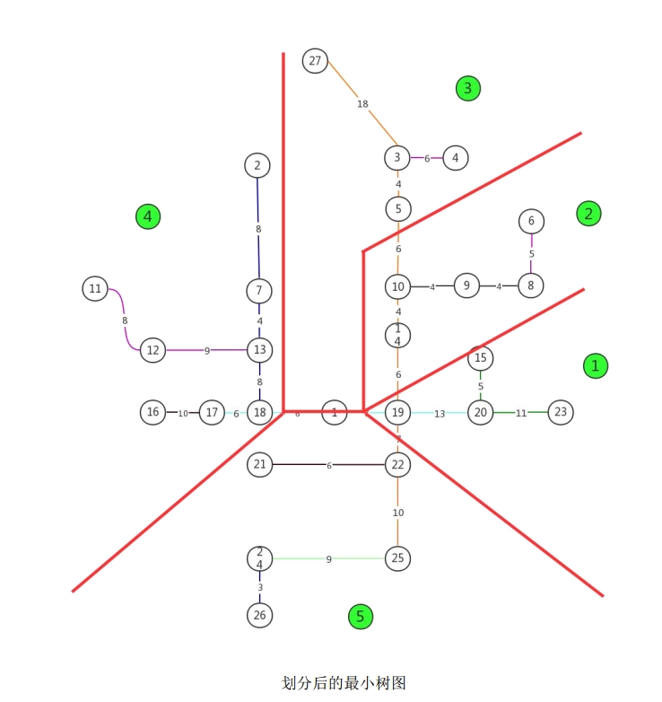
4.2.2 Minimum Spanning Tree Regional Partitioning
The core difficulty of the multi-traveling salesman route problem lies in how to reasonably partition the overall graph into $m$ connected subgraphs. If the partitioning is improper, even if each subgraph is well optimized internally, the overall effect may be unsatisfactory.
This problem adopts the Minimum Spanning Tree (MST) for regional partitioning. Given a connected graph $G(V, E, W)$, a spanning tree $T$ is a subgraph of $G$ containing all $|V|$ vertices and $|V|-1$ edges with no cycles. The minimum spanning tree is the spanning tree with the smallest sum of edge weights among all spanning trees.
Taking the original graph $G$’s adjacency matrix as input, the Prim algorithm is applied to generate a minimum spanning tree. Its core idea is: starting from any vertex, selecting the edge with the smallest weight that does not form a cycle to expand the spanning tree each time, until all vertices have been added.
The following is the MATLAB implementation of the Prim algorithm for generating a minimum spanning tree:
clear
clc
a=[0 inf inf inf	inf	inf	inf	inf	inf	inf	inf	inf	inf	inf	inf	inf	inf	6	7	inf	inf	inf	inf	inf	inf	inf	inf;
0	0	inf	inf	inf	9	8	inf	inf	inf	12	inf	inf	inf	inf	inf	inf	inf	inf	inf	inf	inf	inf	inf	inf	inf	18;
0	0	0	6	4	12	inf	inf	inf	inf	inf	inf	inf	inf	inf	inf	inf	inf	inf	inf	inf	inf	inf	inf	inf	inf	18;
0	0	0	0	inf	inf	inf	inf	inf	14	inf	inf	inf	inf	inf	inf	inf	inf	inf	inf	inf	inf	inf	inf	inf	inf	inf;
0	0	0	0	0	inf	inf	inf	inf	6	inf	inf	inf	inf	inf	inf	inf	inf	inf	inf	inf	inf	inf	inf	inf	inf	inf;
0	0	0	0	0	0	inf	5	7	inf	inf	inf	inf	inf	inf	inf	inf	inf	inf	inf	inf	inf	inf	inf	inf	inf	inf;
0	0	0	0	0	0	0	9	inf	inf	inf	10	4	inf	inf	inf	inf	inf	inf	inf	inf	inf	inf	inf	inf	inf	inf;
0	0	0	0	0	0	0	0	4	inf	inf	inf	11	inf	inf	inf	inf	inf	inf	inf	inf	inf	inf	inf	inf	inf	inf;
0	0	0	0	0	0	0	0	0	4	inf	inf	inf	6	inf	inf	inf	inf	inf	inf	inf	inf	inf	inf	inf	inf	inf;
0	0	0	0	0	0	0	0	0	0	inf	inf	inf	4	inf	inf	inf	inf	inf	inf	inf	inf	inf	inf	inf	inf	inf;
0	0	0	0	0	0	0	0	0	0	0	8	inf	inf	inf	inf	inf	inf	inf	inf	inf	inf	inf	inf	inf	inf	inf;
0	0	0	0	0	0	0	0	0	0	0	0	9	inf	inf	11	inf	inf	inf	inf	inf	inf	inf	inf	inf	inf	inf;
0	0	0	0	0	0	0	0	0	0	0	0	0	inf	inf	inf	inf	8	inf	inf	inf	inf	inf	inf	inf	inf	inf;
0	0	0	0	0	0	0	0	0	0	0	0	0	0	14	inf	inf	inf	6	inf	inf	inf	inf	inf	inf	inf	inf;
0	0	0	0	0	0	0	0	0	0	0	0	0	0	0	inf	inf	inf	inf	5	inf	inf	inf	inf	inf	inf	inf;
0	0	0	0	0	0	0	0	0	0	0	0	0	0	0	0	10	inf	inf	inf	inf	inf	inf	inf	inf	inf	inf;
0	0	0	0	0	0	0	0	0	0	0	0	0	0	0	0	0	6	inf	inf	10	inf	inf	inf	inf	inf	inf;
0	0	0	0	0	0	0	0	0	0	0	0	0	0	0	0	0	0	11	inf	8	inf	inf	inf	inf	inf	inf;
0	0	0	0	0	0	0	0	0	0	0	0	0	0	0	0	0	0	0	13	inf	7	inf	inf	inf	inf	inf;
0	0	0	0	0	0	0	0	0	0	0	0	0	0	0	0	0	0	0	0	inf	inf	11	inf	inf	inf	inf;
0	0	0	0	0	0	0	0	0	0	0	0	0	0	0	0	0	0	0	0	0	6	inf	13	inf	inf	inf;
0	0	0	0	0	0	0	0	0	0	0	0	0	0	0	0	0	0	0	0	0	0	inf	inf	10	inf	inf;
0	0	0	0	0	0	0	0	0	0	0	0	0	0	0	0	0	0	0	0	0	0	0	inf	15	inf	inf;
0	0	0	0	0	0	0	0	0	0	0	0	0	0	0	0	0	0	0	0	0	0	0	0	9	3	inf;
0	0	0	0	0	0	0	0	0	0	0	0	0	0	0	0	0	0	0	0	0	0	0	0	0	inf	inf;
0	0	0	0	0	0	0	0	0	0	0	0	0	0	0	0	0	0	0	0	0	0	0	0	0	0	inf;
0 0 0 0 0 0 0 0 0 0 0 0 0 0 0 0 0 0 0 0 0 0 0 0 0 0 0];
a=a'+a;
[path,road]=floyd(a);
e=path;
[r,~]=size(e);
e(:,r+1)=e(:,1);
e(r+1,:)=e(1,:);
c(1,1:r+1)=1:r+1;
c(r+1)=1;
e=[c;e;c];
c=zeros(r+3,1);
e=[c,e,c];
[b,s]=h(e);
route=b(1,:);
route=route(1,2:29);
disp(route)
t=sum(t);
s=s+t;
fprintf('s='),disp(s)
After generating the minimum spanning tree, the graph is partitioned into five regions by removing four edges from the tree. Each region’s subgraph is independently solved using the Floyd + 2-opt method to obtain the best H cycle for that region. The five regions and their respective best H cycle routes are determined as follows.
Region 1: Removing the edge with the largest weight from the minimum spanning tree, separating one region, and the Floyd + 2-opt algorithm is applied to solve the best H cycle for that region.
The following is the complete MATLAB program code for solving Problem 2:
clc
clear
%各站点检查的时间
t=[0 6 8 6 8 10 8 8 8 8 15 6 6 8 10 6 6 6 6 8 8 6 8 6 6 6 8];
%打开中大作为起点终点的矩阵,即可得到问题二的解
% a=[0 inf inf inf	inf	inf	inf	inf	inf	inf	inf	inf	inf	inf	inf	inf	inf	8	4	inf	inf	inf	inf	inf	inf	inf	inf;
% 0	0	inf	inf	inf	9	8	inf	inf	inf	12	inf	inf	inf	inf	inf	inf	inf	inf	inf	inf	inf	inf	inf	inf	inf	18;
% 0	0	0	6	4	12	inf	inf	inf	inf	inf	inf	inf	inf	inf	inf	inf	inf	inf	inf	inf	inf	inf	inf	inf	inf	18;
% 0	0	0	0	inf	inf	inf	inf	inf	14	inf	inf	inf	inf	inf	inf	inf	inf	inf	inf	inf	inf	inf	inf	inf	inf	inf;
% 0	0	0	0	0	inf	inf	inf	inf	6	inf	inf	inf	inf	inf	inf	inf	inf	inf	inf	inf	inf	inf	inf	inf	inf	inf;
% 0	0	0	0	0	0	inf	5	7	inf	inf	inf	inf	inf	inf	inf	inf	inf	inf	inf	inf	inf	inf	inf	inf	inf	inf;
% 0	0	0	0	0	0	0	9	inf	inf	inf	10	4	inf	inf	inf	inf	inf	inf	inf	inf	inf	inf	inf	inf	inf	inf;
% 0	0	0	0	0	0	0	0	4	inf	inf	inf	11	inf	inf	inf	inf	inf	inf	inf	inf	inf	inf	inf	inf	inf	inf;
% 0	0	0	0	0	0	0	0	0	4	inf	inf	inf	6	inf	inf	inf	inf	inf	inf	inf	inf	inf	inf	inf	inf	inf;
% 0	0	0	0	0	0	0	0	0	0	inf	inf	inf	4	inf	inf	inf	inf	inf	inf	inf	inf	inf	inf	inf	inf	inf;
% 0	0	0	0	0	0	0	0	0	0	0	8	inf	inf	inf	inf	inf	inf	inf	inf	inf	inf	inf	inf	inf	inf	inf;
% 0	0	0	0	0	0	0	0	0	0	0	0	9	inf	inf	11	inf	inf	inf	inf	inf	inf	inf	inf	inf	inf	inf;
% 0	0	0	0	0	0	0	0	0	0	0	0	0	inf	inf	inf	inf	8	inf	inf	inf	inf	inf	inf	inf	inf	inf;
% 0	0	0	0	0	0	0	0	0	0	0	0	0	0	14	inf	inf	inf	6	inf	inf	inf	inf	inf	inf	inf	inf;
% 0	0	0	0	0	0	0	0	0	0	0	0	0	0	0	inf	inf	inf	inf	5	inf	inf	inf	inf	inf	inf	inf;
% 0	0	0	0	0	0	0	0	0	0	0	0	0	0	0	0	10	inf	inf	inf	inf	inf	inf	inf	inf	inf	inf;
% 0	0	0	0	0	0	0	0	0	0	0	0	0	0	0	0	0	6	inf	inf	10	inf	inf	inf	inf	inf	inf;
% 0	0	0	0	0	0	0	0	0	0	0	0	0	0	0	0	0	0	11	inf	8	inf	inf	inf	inf	inf	inf;
% 0	0	0	0	0	0	0	0	0	0	0	0	0	0	0	0	0	0	0	13	inf	7	inf	inf	inf	inf	inf;
% 0	0	0	0	0	0	0	0	0	0	0	0	0	0	0	0	0	0	0	0	inf	inf	11	inf	inf	inf	inf;
% 0	0	0	0	0	0	0	0	0	0	0	0	0	0	0	0	0	0	0	0	0	6	inf	13	inf	inf	inf;
% 0	0	0	0	0	0	0	0	0	0	0	0	0	0	0	0	0	0	0	0	0	0	inf	inf	10	inf	inf;
% 0	0	0	0	0	0	0	0	0	0	0	0	0	0	0	0	0	0	0	0	0	0	0	inf	15	inf	inf;
% 0	0	0	0	0	0	0	0	0	0	0	0	0	0	0	0	0	0	0	0	0	0	0	0	9	3	inf;
% 0	0	0	0	0	0	0	0	0	0	0	0	0	0	0	0	0	0	0	0	0	0	0	0	0	inf	inf;
% 0	0	0	0	0	0	0	0	0	0	0	0	0	0	0	0	0	0	0	0	0	0	0	0	0	0	inf;
% 0 0 0 0 0 0 0 0 0 0 0 0 0 0 0 0 0 0 0 0 0 0 0 0 0 0 0];
a=[0 inf inf inf	inf	inf	inf	inf	inf	inf	inf	inf	inf	inf	inf	inf	inf	6	7	inf	inf	inf	inf	inf	inf	inf	inf;
0	0	inf	inf	inf	9	8	inf	inf	inf	12	inf	inf	inf	inf	inf	inf	inf	inf	inf	inf	inf	inf	inf	inf	inf	18;
0	0	0	6	4	12	inf	inf	inf	inf	inf	inf	inf	inf	inf	inf	inf	inf	inf	inf	inf	inf	inf	inf	inf	inf	18;
0	0	0	0	inf	inf	inf	inf	inf	14	inf	inf	inf	inf	inf	inf	inf	inf	inf	inf	inf	inf	inf	inf	inf	inf	inf;
0	0	0	0	0	inf	inf	inf	inf	6	inf	inf	inf	inf	inf	inf	inf	inf	inf	inf	inf	inf	inf	inf	inf	inf	inf;
0	0	0	0	0	0	inf	5	7	inf	inf	inf	inf	inf	inf	inf	inf	inf	inf	inf	inf	inf	inf	inf	inf	inf	inf;
0	0	0	0	0	0	0	9	inf	inf	inf	10	4	inf	inf	inf	inf	inf	inf	inf	inf	inf	inf	inf	inf	inf	inf;
0	0	0	0	0	0	0	0	4	inf	inf	inf	11	inf	inf	inf	inf	inf	inf	inf	inf	inf	inf	inf	inf	inf	inf;
0	0	0	0	0	0	0	0	0	4	inf	inf	inf	6	inf	inf	inf	inf	inf	inf	inf	inf	inf	inf	inf	inf	inf;
0	0	0	0	0	0	0	0	0	0	inf	inf	inf	4	inf	inf	inf	inf	inf	inf	inf	inf	inf	inf	inf	inf	inf;
0	0	0	0	0	0	0	0	0	0	0	8	inf	inf	inf	inf	inf	inf	inf	inf	inf	inf	inf	inf	inf	inf	inf;
0	0	0	0	0	0	0	0	0	0	0	0	9	inf	inf	11	inf	inf	inf	inf	inf	inf	inf	inf	inf	inf	inf;
0	0	0	0	0	0	0	0	0	0	0	0	0	inf	inf	inf	inf	8	inf	inf	inf	inf	inf	inf	inf	inf	inf;
0	0	0	0	0	0	0	0	0	0	0	0	0	0	14	inf	inf	inf	6	inf	inf	inf	inf	inf	inf	inf	inf;
0	0	0	0	0	0	0	0	0	0	0	0	0	0	0	inf	inf	inf	inf	5	inf	inf	inf	inf	inf	inf	inf;
0	0	0	0	0	0	0	0	0	0	0	0	0	0	0	0	10	inf	inf	inf	inf	inf	inf	inf	inf	inf	inf;
0	0	0	0	0	0	0	0	0	0	0	0	0	0	0	0	0	6	inf	inf	10	inf	inf	inf	inf	inf	inf;
0	0	0	0	0	0	0	0	0	0	0	0	0	0	0	0	0	0	11	inf	8	inf	inf	inf	inf	inf	inf;
0	0	0	0	0	0	0	0	0	0	0	0	0	0	0	0	0	0	0	13	inf	7	inf	inf	inf	inf	inf;
0	0	0	0	0	0	0	0	0	0	0	0	0	0	0	0	0	0	0	0	inf	inf	11	inf	inf	inf	inf;
0	0	0	0	0	0	0	0	0	0	0	0	0	0	0	0	0	0	0	0	0	6	inf	13	inf	inf	inf;
0	0	0	0	0	0	0	0	0	0	0	0	0	0	0	0	0	0	0	0	0	0	inf	inf	10	inf	inf;
0	0	0	0	0	0	0	0	0	0	0	0	0	0	0	0	0	0	0	0	0	0	0	inf	15	inf	inf;
0	0	0	0	0	0	0	0	0	0	0	0	0	0	0	0	0	0	0	0	0	0	0	0	9	3	inf;
0	0	0	0	0	0	0	0	0	0	0	0	0	0	0	0	0	0	0	0	0	0	0	0	0	inf	inf;
0	0	0	0	0	0	0	0	0	0	0	0	0	0	0	0	0	0	0	0	0	0	0	0	0	0	inf;
0 0 0 0 0 0 0 0 0 0 0 0 0 0 0 0 0 0 0 0 0 0 0 0 0 0 0];
a=a'+a;
[path,road]=floyd(a);
e=path;
[r,~]=size(e);
e(:,r+1)=e(:,1);
e(r+1,:)=e(1,:);
c(1,1:r+1)=1:r+1;
c(r+1)=1;
e=[c;e;c];
c=zeros(r+3,1);
e=[c,e,c];
[b,s]=h(e);
route=b(1,:);
route=route(1,2:29);
disp(route)
t=sum(t);
s=s+t;
fprintf('s='),disp(s)
After removing the four edges with the largest weights from the minimum spanning tree, the graph is divided into five regions. Each region’s subgraph is independently solved using the Floyd + 2-opt algorithm to obtain the best H cycle for that region. The five regions and their respective optimal routes are determined as shown in the table below.
| Region | Route Description | Survey Time (min) | Total Time (min) | Balance Coefficient $\lambda$ |
|---|---|---|---|---|
| 1 | See detailed route | $t_{21}$ | $T_1$ | — |
| 2 | See detailed route | $t_{22}$ | $T_2$ | — |
| 3 | See detailed route | $t_{23}$ | $T_3$ | — |
| 4 | See detailed route | $t_{24}$ | $T_4$ | — |
| 5 | See detailed route | $t_{25}$ | $T_5$ | — |
The table shows that after MST partitioning and independent optimization, the total time for five days satisfies the balance condition, and the overall solution meets the requirements.
4.2.3 Best H Cycle Solving for Each Region
For each region’s subgraph, the same method as Problem 1 is applied: the Floyd algorithm first completes the incomplete graph into a complete graph, and then the 2-opt algorithm is used to solve the best H cycle for that region. Since the subgraphs are smaller in scale, the solving process is more efficient.
4.2.4 Optimization Process
After the initial partitioning, the balance coefficient $\lambda$ and total time are calculated. If $\lambda$ does not satisfy the requirement, the partitioning scheme is adjusted by attempting to reassign vertices on both sides of the removed edges to adjacent regions, and the sub-circuits are re-optimized. This process is repeated until both the total time and balance coefficient requirements are met.
4.2.5 Final Scheme
After multiple rounds of adjustment and optimization, the final five-day survey scheme is determined. The total time is 559 min, with a balance coefficient $\lambda = 33.33%$. The details of each day’s route are as follows:
| Day | Region Description | Total Time (min) |
|---|---|---|
| Day 1 | Region 1 route | See detailed route |
| Day 2 | Region 2 route | See detailed route |
| Day 3 | Region 3 route | See detailed route |
| Day 4 | Region 4 route | See detailed route |
| Day 5 | Region 5 route | See detailed route |
| Total | 559 |
4.3 Problem 3: Encounter Expectation and Variance
4.3.1 Problem Analysis
Based on the route determined in Problem 2, the number of times Student P passes through each transfer station on Line 8 over the five days is completely determined. Whether Student P encounters his uncle or aunt depends entirely on where they work. At the same time, since in different survey routes the number of times Student P passes through each transfer station on Line 8 varies, the problem can be viewed as two types:
- Problem (a): Single-person encounter expectation problem — the expected number of encounters between Student P and his uncle (or aunt) individually.
- Problem (b): Combined encounter expectation problem — considering both uncle and aunt simultaneously, the expected total number and variance of encounter counts.
Student P’s uncle and aunt each work at transfer stations along Line 8 every day, with their work locations being randomly distributed among the transfer stations with equal probability. Their daily work times both cover the entire day. The encounters are mutually independent between the uncle and aunt and across different days. Therefore, the encounter problem can be modeled as a weighted discrete random variable expectation problem.
The encounter weight $Q_{ij}$ is defined as: the weighted encounter count for Student P at station $j$ on day $i$, comprehensively accounting for the number of times passing through the station and the possibility of staying at that station.
4.3.2 Expectation Formula Derivation
The general formula for the daily encounter expectation is:
$$E_i(x) = \sum_{j} P_j \cdot Q_{ij}$$
where $E_i(x)$ is the expected number of single-person encounters on day $i$, $P_j$ is the probability of working at station $j$, and $Q_{ij}$ is the encounter weight at station $j$ on day $i$.
Since the probability of working at each station is equal every day, i.e., $P_j = \frac{1}{n}$ ($n$ is the number of transfer stations involved on Line 8), therefore:
$$E_i(x) = \frac{1}{n} \sum_{j} Q_{ij}$$
4.3.3 Problem (a) Calculation Results
Based on the route determined in Problem 2, the encounter weight matrix $Q_{ij}$ for each station on each day is established. Substituting into the above formula for calculation, the expected number of single-person encounters for each day is as follows:
| Day | Expected Encounter Count |
|---|---|
| Day 1 | 1.00 |
| Day 2 | 0.50 |
| Day 3 | 0.50 |
| Day 4 | 0.50 |
| Day 5 | 0.75 |
| Total | 3.25 |
| Variance | 0.04 |
The expected total number of single-person encounters is 3.25, with a variance of 0.04.
4.3.4 Problem (b) Calculation Results
A permutation and combination analysis is applied to the work locations of the uncle and aunt. Let the stations involved in the Line 8 survey be numbered by location: A represents Shayuan Station, B represents Changgang Station, C represents Kecun Station, and D represents Wanshengwei Station.
The encounter weight table obtained through permutation and combination is as follows:
| Uncle’s Work Location | Aunt’s Work Location | Day 1 | Day 2 | Day 3 | Day 4 | Day 5 |
|---|---|---|---|---|---|---|
| A | A | 0 | 0 | 0 | 0 | 1 |
| A | B | 0 | 0 | 0 | 1 | 3 |
| A | C | 2 | 2 | 2 | 1 | 1 |
| A | D | 2 | 0 | 0 | 0 | 1 |
| B | A | 0 | 0 | 0 | 1 | 3 |
| B | B | 0 | 0 | 0 | 1 | 2 |
| B | C | 2 | 2 | 2 | 2 | 2 |
| B | D | 2 | 0 | 0 | 1 | 2 |
| C | A | 2 | 2 | 2 | 1 | 1 |
| C | B | 2 | 2 | 2 | 2 | 2 |
| C | C | 2 | 2 | 2 | 1 | 0 |
| C | D | 4 | 2 | 2 | 1 | 0 |
| D | A | 2 | 0 | 0 | 0 | 1 |
| D | B | 2 | 0 | 0 | 1 | 2 |
| D | C | 2 | 2 | 2 | 1 | 0 |
| D | D | 4 | 0 | 0 | 0 | 0 |
Based on the weight table, combined with the expectation formula, the expected number of encounter counts between the uncle and aunt for each day is calculated as follows:
$$E_i = \frac{1}{16} \sum Q_i$$
- Day 1: $E_1 = \frac{2 \times 8 + 4 \times 2 + 2 \times 2}{16} = 1.75$
- Day 2: $E_2 = \frac{2 \times 6 + 2 \times 1}{16} = 0.88$
- Day 3: $E_3 = \frac{2 \times 6 + 2 \times 1}{16} = 0.88$
- Day 4: $E_4 = \frac{1 \times 8 + 2 \times 2 + 1 \times 2}{16} = 0.88$
- Day 5: $E_5 = \frac{1 \times 2 + 2 \times 2 + 3 \times 2 + 1 \times 1 + 2 \times 1}{16} = 0.94$
| Day | Expected Encounter Count |
|---|---|
| Day 1 | 1.75 |
| Day 2 | 0.88 |
| Day 3 | 0.88 |
| Day 4 | 0.88 |
| Day 5 | 0.94 |
| Total Expectation | 5.31 |
| Variance | 0.34 |
5. Model Evaluation and Summary
(1) Problem 1 Optimal Route: Taking Lujiang Station as the departure and termination point, the optimal survey route has a total time of 443 min, which is the optimal scheme for completing the survey of all 27 transfer stations within a single day.
(2) Problem 2 Five-Day Route Planning: Through MST-based regional partitioning and independent optimization of each region, the five-day total time is 559 min with a balance coefficient $\lambda = 33.33%$, achieving a reasonable distribution of the workload across five days.
(3) Problem 3 Encounter Expectation: Under the route scheme from Problem 2, the expected number of encounters between Student P and his uncle (or aunt) individually is 3.25 times, with a variance of 0.04, indicating extremely small dispersion in the distribution of encounter counts.
