
Chapter 0: Technology stack and Python library description
0.1 Technology stack overview
This project as a whole is a typical risk control modeling solution of “offline feature engineering + machine learning modeling + business strategy implementation”. The core technology stack is mainly divided into three layers:
-
Data processing layer Use Spark / PySpark to complete large-scale sample processing, feature splicing, time window aggregation and batch export, supporting the calculation of massive features in a distributed environment.
-
Analytical Modeling Layer Use Python as the main modeling language, combined with pandas, numpy, scikit-learn, lightgbm, toad and other libraries to complete sample processing, feature screening, model training, parameter tuning and effect evaluation.
-
Business Application Layer Transform the model output results into implementable collection and screening strategies, including the first round of detection of the main model, dynamic recovery of the auxiliary model, and the final resource allocation strategy based on ROI.
0.2 The main technologies this project relies on
From the perspective of full-text code implementation, the project mainly relies on the following technical components:
- Python: core development language
- Spark/PySpark: Offline feature engineering and distributed data processing
- LightGBM: Main model training and feature importance ranking
- scikit-learn: Dataset partitioning, grid search and model evaluation
- toad: Feature screening, IV calculation, risk control modeling auxiliary analysis
- pandas/numpy: Structured data processing and numerical calculations
Chapter 1: Project Background and Business Issues
1.1 Definition of long-aging orders and industry pain points
In credit business, post-loan management is the last link in the closed loop of risk control. When an order enters the overdue stage, the allocation of collection efforts directly determines the input-output ratio of labor costs.
The so-called “long-aging orders” are defined in this project as the user group who are 15 days or more overdue and have not yet repaid. These users have the following common characteristics:
- Low willingness to repay: Still refuses to repay after more than 15 days of continuous collection pressure, and the subjective willingness to repay has significantly declined;
- High Difficulty in Collection: Conventional text messages and telephone collections have limited impact on it, so collectors need to invest more energy;
- Positive samples are extremely sparse: Only a small number of users can finally successfully repay after more than 15 days of collection, and the data distribution is seriously skewed.
1.2 Three major problems with the existing reminder model
Before the introduction of machine learning modeling, the business side used the full collection mode for long-aging orders—that is, uniformly arranging manpower for collection of all long-aging orders. There are three core problems with this approach:
Problem 1: Huge labor costs
The volume of long-aged orders is large and continues to accumulate. If manual collection is invested in each order, labor costs will increase linearly. The collection team needs to continue to expand, but the increase in collection amount cannot keep up with the increase in manpower investment.
Problem 2: ROI is extremely low
The overall labor ROI (collection amount / labor cost) of the reminder model has been hovering between 1.1 and 1.5 for a long time, and the collection efficiency is only 5%. After deducting capital costs and operating costs, this number has almost no profit margin, or even losses.
Problem 3: Affects team morale
Collection agents make a large number of calls every day, and most of the people they come into contact with are users who refuse to repay or even have bad attitudes. The success rate is extremely low. If this continues for a long time, the team will easily feel exhausted, the turnover rate will increase, and the overall collection efficiency will further decline, forming a vicious cycle.
1.3 Project Goal: From “Full Quantity Clearance” to “Accurate Detection + Dynamic Retrieval”
Based on the above pain points, the core issues are:
**Is it possible to automatically identify orders with high callback potential from a large number of long-aged orders, and continue to recover orders with callback value as the stages advance, so that limited manpower can focus on the highest-value cases? **
Specific business goals are:
| index | Communicate the current situation | target value |
|---|---|---|
| People ROI | 1.1~1.5 | > 2.0 |
| recall efficiency | 5% | >10% |
| Collection strategies | Full reminder | Accurate detection of main model + dynamic recovery of auxiliary model |
The overall idea of the project is as follows:
- Feature construction: Integrate multi-dimensional data such as user login, APP behavior, device information, SMS content, basic information, etc., and build a massive feature library (approximately 10,000 dimensions) based on the five-dimensional cross combination of order type × behavior label × time dimension × indicator value × calculation method;
- Multiple rounds of feature screening: IV value initial screening (empty=0.6, iv=0.05, corr=0.8) → LGBM gain value stability re-screening (5 times of random modeling × Top100 intersection) → LGBM Top60 convergence, and finally retain about 60 high-value features;
- LGBM prediction model construction: Taking “whether there is repayment during the user stage” as the label (repayment = 1, non-repayment = 0), train the main model, and perform the first round of sorting and detection of long-aging orders;
- Auxiliary model dynamic retrieval: Based on the new behavioral signals in the stage, secondary identification of orders not detected by the main model is carried out, focusing on capturing orders that have become stronger again such as login, repayment of other orders, partial repayment, etc.;
- ROI-oriented implementation: Form a combined strategy of “first-round inspection of main model + dynamic supplement of auxiliary models” to continuously improve inspection quality and recovery output while reducing manpower investment.
Chapter 2: Data source and feature engineering system
2.1 Data source panorama
The data sources of this project cover four dimensions: user application behavior, credit performance, post-loan collection interaction, and full-link behavior within the APP. All data involving user privacy is legally authorized through the Google Store channel, and can only be collected with the user’s consent.
(1) User information
The data captured with the user’s authorization when applying for an order includes three sub-modules:
- APP List: The list of applications installed on the user’s mobile phone, obtained through the Google Store channel, can reflect the user’s living and consumption habits, financial demand density, etc.;
- Device information: Device parameters when applying for an order, including device model, brand, operating system version, etc., used to determine the stability of the user’s device and whether there are risky behaviors such as multi-device switching;
- SMS message: The text message content extracted in a structured manner after user authorization, mainly covering bank repayment reminder text messages, external loan platform text messages, etc., which can reflect the user’s debt pressure and financial tightness;
- Basic personal information: Identity information that users actively fill in during the application process, including age, occupation, education and other demographic fields.
(2) Risk dimension
Credit indicators provided by external data sources when users apply for orders, including:
- Multiple application risk situation: The user’s application records on multiple credit platforms reflect the risk of over-indebtedness;
- Credit Rating: The comprehensive credit score grade given by external credit reporting or data partners directly reflects the user’s historical credit performance.
(3) Collection information
The user’s post-loan collection data before entering the long account aging stage includes historical collection records before collection, collection methods (text messages/phone calls/outside visits), historical collection results, etc. The reminder information can help the model learn: before entering the long aging period, which collection behavior patterns are related to the final repayment results.
(4) User behavior information
The user’s full-link operation log within the APP interface is the most granular behavioral data source for this project:
- Registration behavior: registration time, registration channel, registration equipment, etc.;
- Login behavior: login time, login frequency, login device changes, login region changes, etc.;
- Button clicks: distribution of click hot spots on each functional page, page dwell time, page jump path, application process interruption nodes, etc.;
- APP behavioral data can capture the user’s active participation in the product, and deep-seated behaviors (such as proactively checking the repayment plan) are often highly correlated with repayment willingness.
2.2 Engineering construction of feature dimensions
If a single behavior field is not cross-combined through time windows, the effect of directly entering the model is often very poor. For example: “Number of logins in the past 7 days” has a much stronger discriminating ability than “Total number of logins in history” in long account aging scenarios, because recent behavior can better reflect the user’s current willingness to repay.
The feature construction of this project adopts an engineering scheme of five-dimensional cross combination of Order Type × Behavior Label × Time Dimension × Indicator Value × Calculation Method. Take Multi-head application feature as an example to fully explain the feature naming specifications and construction logic.
2.2.1 Feature naming convention
userMulti{订单类型}{行为标签}{指标值}{计算方式}{时间窗口}D
Feature names directly carry business meaning, and calibers can be understood without additional documentation:
| Feature name | meaning |
|---|---|
userMultiAllAllOrderCnt7D |
Number of requests for all orders in the past 7 days |
userMultiIsLoanAllAmountSum30D |
The total amount of disbursed orders in the past 30 days |
userMultiIsNoLoanPackageDistinctCnt14D |
The number of different products involved in undisbursed orders in the past 14 days |
2.2.2 Three dimensions of feature construction
Dimension one: time dimension
Divided according to the number of days from the application time to the sample point: 1D, 3D, 7D, 14D, 30D, 60D, All.
Dimension 2: Order type
Filter subsamples by user historical order status:
| Order type | meaning |
|---|---|
All |
Full historical orders |
IsLoan |
Orders that have been successfully loaned in history |
IsNoLoan |
Orders applied for but not released in history |
Dimension three: behavioral labeling
Further refined screening based on order type:
| behavior tag | meaning |
|---|---|
All |
No additional filtering |
Overdue1Day |
Orders overdue for ≥1 day |
Overdue3Day |
Orders overdue for ≥3 days |
PreRepay3Day |
Orders with repayment ≥3 days in advance |
2.2.3 Indicator values and calculation methods
Indicator value (cal_field): Key fields covering the entire life cycle of historical orders:
| indicator value | meaning |
|---|---|
Package |
Product applied for |
Order |
Order ID |
Amount |
loan amount |
ApplyLendingInterval / ApplyRepaidInterval |
Time interval of each node |
OverdueDay/PreRepayDay |
Number of days overdue/number of days in advance of repayment |
PartRepayAmt/PartRepayAmtPct |
Partial repayment amount and proportion |
Calculation method: 12 types in total, reused for all indicator values:
| Calculation method | meaning |
|---|---|
Cnt |
times/number of transactions |
DistinctCnt |
number of different values |
RepeatCnt |
Number of repetitions (= Cnt - DistinctCnt) |
Sum |
Sum |
Avg |
mean |
Max |
maximum value |
Min |
minimum value |
Std |
population standard deviation |
Skew |
Skewness |
Median |
median |
Pct |
Ratio of specified conditions/full conditions |
DistinctPct |
Proportions of different values |
Feature generation formula:
特征 = 订单类型 + 行为标签 + 指标值 + 计算方式 + 时间窗口
Example interpretation: userMultiAllAllOrderCnt7D
- Order type All (full quantity order)
- Behavior Tags All (no additional filtering)
- Indicator value Order
- Calculation method Cnt (count)
- Time window 7D (last 7 days)
2.2.4 Portfolio size estimation
订单类型(N) × 行为标签(M) × 时间窗口(T) × 指标值(K) × 计算方式(A)
= N × M × T × K × A 个特征
Take multi-head application features as an example, assuming there are 3 order types, 10 behavior labels, 7 time windows, 10 indicator values, and 12 calculation methods, a single long-head application module can generate 3 × 10 × 7 × 10 × 12 = 25200 feature dimensions.
The same logic is applied to all data sources such as user information, risk dimensions, collection information, user behavior information, etc., and finally a massive feature library is built.
2.3 Missing value and outlier processing strategies
Among the massive features, the sources of null values in the original data are complicated—it may be due to unauthorized user authorization, collection failure, or unrecorded status in the business. This project adopts the strategy of multi-level coding + exclusionary aggregation instead of a simple filling method.
2.3.1 Multi-level null coding system
An additional {indicator value}_none tag column is generated for each original field, and the following situations are uniformly recognized as null value tags through the get_is_none function:
def get_is_none(x):
    if x is None or str(x).replace(' ','').lower().strip() in ['-999999','-999976','-999977','-999978',
                                                               '-999999.0','-999999.0000', '-999976.0','-999976.0000',
                                                               '-999977.0','-999977.0000', '-999978.0','-999978.0000',
                                                               'none','nan','nat','','000000000000000']:
        return 1
    else:
        return 0
u_get_is_none = udf(get_is_none, IntegerType())
At the same time, different coding values are assigned to different abnormal situations, and different business meanings can be distinguished during model training:
| coding | meaning |
|---|---|
-999976 |
Calculation exception (system error such as type conversion failure) |
-999977 |
The dividend is empty or the divisor is empty |
-999978 |
Divisor is 0 |
-999999 |
Null value at the business level (if the user did not actually perform any action) |
2.3.2 Exclusive aggregation
When generating aggregate features, force filter records with {metric value}_none == 1 in the conditions of each aggregation calculation:
if condition_label == 'All':
    cal_condition = (f.col(time_field) <= time_windows_value) & (f.col(time_field) >= 0) & (f.col(f'{cal_field}_none') == 0 )
else:
    cal_condition = (f.col(time_field) <= time_windows_value) & (f.col(time_field) >= 0) & (f.col(f'{cal_field}_none') == 0 ) & (f.col(f'type_{condition_label}') == 1)
This means: all aggregate features (Cnt/Sum/Avg/Max, etc.) are calculated based on valid records rather than being shoehorned into the model with uniform padding values.
2.3.3 Project implementation logic
The actual process is two steps:
Step 1: For each original indicator value field, generate the corresponding _none tag column:
for cal_field in cal_field_list:
    relative_df = relative_df.withColumn(f'{cal_field}_none', u_get_is_none(cal_field))
Step 2: During aggregation calculation, add the _none == 0 restriction to the aggregation condition of each aggregation indicator to ensure that null value records do not participate in any mathematical operations and ensure the quality of features from the source.
2.4 Technical implementation: Spark-based feature engineering pipeline
This section introduces the whole process of how to extract raw data from the database based on Spark, and finally generate features through UDF processing and multi-dimensional aggregation. The codes are all taken from the real project ipynb implementation.
2.4.1 Core UDF definition
The following are the core custom functions in ipynb, used for time processing, null value judgment and calculation of key business indicators:
(1) Null value judgment and division safety
def get_is_none(x):
    if x is None or str(x).replace(' ','').lower().strip() in ['-999999','-999976','-999977','-999978',
                                                               '-999999.0','-999999.0000', '-999976.0','-999976.0000',
                                                               '-999977.0','-999977.0000', '-999978.0','-999978.0000',
                                                               'none','nan','nat','','000000000000000']:
        return 1
    else:
        return 0
u_get_is_none = udf(get_is_none, IntegerType())

def get_cal_division(numerator, denominator):
    try:
        if denominator == 0:
            return -999978
        elif get_is_none(numerator) or get_is_none(denominator):
            return -999977
        else:
            return round(numerator / denominator, 2)
    except Exception as e:
        return -999976
(2) Time zone conversion
def remove_tz(date_time):
    return datetime.strptime(date_time.strftime('%Y-%m-%d %H:%M:%S'), '%Y-%m-%d %H:%M:%S')

def convert_to_nigeria_time(date_time):
    if type(date_time) == str:
        date_time_d = str(date_time)[0:19]
    else:
        date_time_d = date_time.strftime('%Y-%m-%d %H:%M:%S')
    time_stamp = time.mktime(time.strptime(date_time_d, '%Y-%m-%d %H:%M:%S'))
    utc_dt = datetime.utcfromtimestamp(time_stamp).replace(tzinfo=pytz.utc)
    dest_tz = timezone('Africa/Lagos')
    dest_dt = dest_tz.normalize(utc_dt.astimezone(dest_tz))
    return remove_tz(dest_dt)

def change_to_nigeria(date_time):
    if get_is_none(date_time):
        return None
    else:
        return convert_to_nigeria_time(date_time)

u_change_to_nigeria = udf(change_to_nigeria, TimestampType())
(3) Time interval calculation
def get_timedelta_strtime(time_end, time_start):
    try:
        if get_is_none(time_end) or get_is_none(time_start):
            return None
        if len(str(time_end)) < 15 and len(str(time_start)) < 15:
            time_start = datetime.strptime(str(time_start)[0:10], "%Y-%m-%d")
            time_end = datetime.strptime(str(time_end)[0:10], "%Y-%m-%d")
        elif len(str(time_end)) < 15 and len(str(time_start)) > 15:
            time_start = datetime.strptime(str(time_start)[0:19], "%Y-%m-%d %H:%M:%S")
            time_end = datetime.strptime(str(time_end)[0:10], "%Y-%m-%d")
        else:
            time_start = datetime.strptime(str(time_start)[0:19], "%Y-%m-%d %H:%M:%S")
            time_end = datetime.strptime(str(time_end)[0:19], "%Y-%m-%d %H:%M:%S")
        seconds = (time_end - time_start).total_seconds()
        if seconds < 0:
            seconds = None
        return seconds
    except Exception as e:
        return -999976

u_get_timedelta_strtime = udf(get_timedelta_strtime, FloatType())
(4) Calculation of days for early repayment
def get_pre_repay_day(real_repay_time, due_time, is_repay):
    if str(is_repay) in ['1', '1.0']:
        if get_is_none(real_repay_time):
            return -999999
        elif get_is_none(due_time):
            return -999999
        else:
            real_repay_time = datetime.strptime(str(real_repay_time)[0:10], "%Y-%m-%d")
            due_time = datetime.strptime(str(due_time)[0:10], "%Y-%m-%d")
            pre_repayday = int((due_time - real_repay_time).days)
            if pre_repayday < 0:
                pre_repayday = -999999
            return pre_repayday
    else:
        return -999999

u_get_pre_repay_day = udf(get_pre_repay_day, IntegerType())
2.4.2 Core aggregate function: get_agg_v2
This function encapsulates 12 types of aggregation calculation logic, automatically constructs Spark aggregation expressions after inputting five-dimensional parameters, and is the core of the entire feature engineering pipeline:
def get_agg_v2(time_field, dt_, condition_label, condition_type, cal_field, cal_type, fea_name):
    """
    聚合函数
    :param time_field:
    :param dt_:
    :param contact_condition:
    :param cal_field:
    :param cal_type:
    :return:
    """
    print(f"export feature:{fea_name}")
    if dt_ != 'All':
        time_windows_value = dt_ * 24 * 60 * 60
    else:
        time_windows_value = 1000 * 24 * 60 * 60

    if condition_label == 'All':
        cal_condition = (f.col(time_field) <= time_windows_value) & (f.col(time_field) >= 0) & (f.col(f'{cal_field}_none') == 0)
    else:
        cal_condition = (f.col(time_field) <= time_windows_value) & (f.col(time_field) >= 0) & (f.col(f'{cal_field}_none') == 0) & (f.col(f'type_{condition_label}') == 1)

    if condition_type != 'All':
        cal_condition = cal_condition & (f.col(f'type_{condition_type}') == 1)

    if cal_type == 'Std':
        return f.stddev_pop(f.when(cal_condition, f.col(cal_field))).alias(fea_name)
    elif cal_type == 'Avg':
        return f.mean(f.when(cal_condition, f.col(cal_field))).alias(fea_name)
    elif cal_type == 'Sum':
        return f.sum(f.when(cal_condition, f.col(cal_field))).alias(fea_name)
    elif cal_type == 'sumDistinct':
        return f.sumDistinct(f.when(cal_condition, f.col(cal_field))).alias(fea_name)
    elif cal_type == 'Max':
        return f.max(f.when(cal_condition, f.col(cal_field))).alias(fea_name)
    elif cal_type == 'Skew':
        return f.skewness(f.when(cal_condition, f.col(cal_field))).alias(fea_name)
    elif cal_type == 'Median':
        return f.percentile_approx(f.when(cal_condition, f.col(cal_field)), 0.5).alias(fea_name)
    elif cal_type == 'Min':
        return f.min(f.when(cal_condition, f.col(cal_field))).alias(fea_name)
    elif cal_type == 'Cnt':
        return f.count(f.when(cal_condition, f.col(cal_field))).alias(fea_name)
    elif cal_type == 'DistinctCnt':
        return f.countDistinct(f.when(cal_condition, f.col(cal_field))).alias(fea_name)
    elif cal_type == 'RepeatCnt':
        return (f.count(f.when(cal_condition, f.col(cal_field))) - f.countDistinct(f.when(cal_condition, f.col(cal_field)))).alias(fea_name)
    elif cal_type == 'DistinctPct':
        all_condition = (f.col(time_field) <= time_windows_value) & (f.col(time_field) >= 0) & (f.col(f'{cal_field}_none') == 0)
        return (f.countDistinct(f.when(cal_condition, f.col(cal_field))) / f.countDistinct(f.when(all_condition, f.col(cal_field)))).alias(fea_name)
    elif cal_type == 'Pct':
        all_condition = (f.col(time_field) <= time_windows_value) & (f.col(time_field) >= 0) & (f.col(f'{cal_field}_none') == 0)
        return (f.count(f.when(cal_condition, f.col(cal_field))) / f.count(f.when(all_condition, f.col(cal_field)))).alias(fea_name)
    elif cal_type == 'RepeatPct':
        all_condition = (f.col(time_field) <= time_windows_value) & (f.col(time_field) >= 0) & (f.col(f'{cal_field}_none') == 0)
        return ((f.count(f.when(cal_condition, f.col(cal_field))) - f.countDistinct(f.when(cal_condition, f.col(cal_field))))
                / (f.count(f.when(all_condition, f.col(cal_field))) - f.countDistinct(f.when(all_condition, f.col(cal_field))))).alias(fea_name)

    return None
2.4.3 Data preprocessing + aggregate feature generation
The core encapsulation class of the entire pipeline includes two methods: data preprocessing (prepare_df) and batch aggregation (feature_df):
class Features1(object):

    def __init__(self, spark: SparkSession):
        self.spark = spark

    def prepare_df(self, from_sample, prepare_table):
        # 加载订单表
        self.spark.sql(f""" select * from
                risk.dw_order_info_slice_2
                where
                country = 'NIGERIA'
                and merchant_id = 1
                and not isnull(APPLY_DAY)
            """) \
            .createOrReplaceTempView('loan_df')

        col_list = self.spark.sql("select * from risk.dw_order_info_slice_2").columns
        col_list.remove('REPAY_TIME_FORMAT')
        col_list = [f"o.{x} as SAMPLE_{x}" for x in col_list]

        # 关联样本表与订单表
        self.spark.sql(f"""
            select {','.join(col_list)}, s.due_day as SAMPLE_REPAY_TIME_FORMAT,
            to_date(s.d14_date) as SAMPLE_d14_date,
            date_add(to_date(s.d14_date), 1) as SAMPLE_APPLY_LIMIT_DAY
            from
            {from_sample} s left join risk.dw_order_info_slice_2 o
            on s.bis_order_id = o.bis_order_id
            where
            country = 'NIGERIA' and merchant_id = 1
        """).createOrReplaceTempView('sample_order')

        self.spark.sql("""
            select s.* , l.* from
            sample_order s left join loan_df l
            on s.SAMPLE_BIS_USER_ID = l.BIS_USER_ID
            where
            l.APPLY_DAY < S.SAMPLE_APPLY_LIMIT_DAY
            and  S.SAMPLE_APPLY_TIME < l.APPLY_TIME
            and s.SAMPLE_BIS_ORDER_ID != l.BIS_ORDER_ID
        """).createOrReplaceTempView('sample_df')

        relative_df = self.spark.sql("select * from sample_df")

        # 时区转换
        relative_df = relative_df.withColumn('LENDING_TIME_FORMAT', u_get_time_process('LENDING_TIME_FORMAT', 'SAMPLE_APPLY_LIMIT_DAY'))
        relative_df = relative_df.withColumn('REPAIED_TIME_FORMAT', u_get_time_process('REPAIED_TIME_FORMAT', 'SAMPLE_APPLY_LIMIT_DAY'))
        relative_df = relative_df.withColumn('SAMPLE_APPLY_TIME_NI', u_change_to_nigeria('SAMPLE_APPLY_TIME'))
        relative_df = relative_df.withColumn('LENDING_TIME_TIMESTAMP_NI', u_change_to_nigeria('LENDING_TIME_FORMAT'))
        relative_df = relative_df.withColumn('REPAIED_TIME_TIMESTAMP_NI', u_change_to_nigeria('REPAIED_TIME_FORMAT'))
        relative_df = relative_df.withColumn('APPLY_TIME_NI', u_change_to_nigeria('APPLY_TIME'))
        relative_df = relative_df.withColumn('SAMPLE_APPLY_DAY_NI', u_get_date_from_timestamp('SAMPLE_APPLY_TIME_NI'))

        # 生成时间间隔字段(秒)
        relative_df = relative_df.withColumn('ApplyLendingInterval', u_get_timedelta_strtime('LENDING_TIME_TIMESTAMP_NI', 'SAMPLE_APPLY_TIME_NI'))
        relative_df = relative_df.withColumn('ApplyApplyInterval', u_get_timedelta_strtime('APPLY_TIME_NI', 'SAMPLE_APPLY_TIME_NI'))
        relative_df = relative_df.withColumn('ApplyRepaiedInterval', u_get_timedelta_strtime('REPAIED_TIME_TIMESTAMP_NI', 'SAMPLE_APPLY_TIME_NI'))
        relative_df = relative_df.withColumn('LimitApplyInterval', u_get_timedelta_strtime('SAMPLE_APPLY_LIMIT_DAY', 'APPLY_TIME'))

        # 生成业务标签字段
        relative_df = relative_df.withColumn('is_reject', u_get_value_equals(30)(col('STATUS')))
        relative_df = relative_df.withColumn('is_cancel', u_get_value_equals(60)(col('STATUS')))
        relative_df = relative_df.withColumn('is_loan', u_get_is_loan('LENDING_TIME_TIMESTAMP_NI', 'SAMPLE_APPLY_LIMIT_DAY'))
        relative_df = relative_df.withColumn('is_repay', u_get_is_repay('REPAIED_TIME_TIMESTAMP_NI'))

        # 生成日期字段
        relative_df = relative_df.withColumn('ApplyDays', u_get_message_day('APPLY_TIME_NI'))
        relative_df = relative_df.withColumn('LendingDays', u_get_message_day('LENDING_TIME_TIMESTAMP_NI'))
        relative_df = relative_df.withColumn('RepayDays', u_get_message_day('REPAIED_TIME_TIMESTAMP_NI'))
        relative_df = relative_df.withColumn('repay_date', u_get_message_day('REPAIED_TIME_TIMESTAMP_NI'))
        relative_df = relative_df.withColumn('due_date', u_get_message_day('ORG_REPAY_TIME'))
        relative_df = relative_df.withColumn('PreRepayDay', u_get_pre_repay_day('repay_date', 'due_date', 'is_repay'))

        # 生成实还金额、部分还款相关字段
        relative_df = relative_df.withColumn('REPAIED_AMOUNT_FIX', u_get_repaid_amount('REPAY_AMOUNT', 'REPAIED_AMOUNT', 'is_repay'))
        relative_df = relative_df.withColumn('REPAIED_AMOUNT_FIX', get_none_defalut_value(0)(col('REPAIED_AMOUNT_FIX')))
        relative_df = relative_df.withColumn('REPAY_AMOUNT', get_none_defalut_value(0)(col('REPAY_AMOUNT')))
        relative_df = relative_df.withColumn('IsPartRepay', u_is_part_repay('is_repay', 'REPAIED_AMOUNT_FIX', 'REPAY_AMOUNT'))
        relative_df = relative_df.withColumn('PartRepayAmtPct', u_get_part_repay_amount_pct('is_repay', 'REPAIED_AMOUNT_FIX', 'REPAY_AMOUNT'))
        relative_df = relative_df.withColumn('PartRepayAmt', u_get_part_repay_amount('IsPartRepay', 'REPAIED_AMOUNT_FIX', 'REPAY_AMOUNT'))

        # 生成布尔标签字段
        relative_df = relative_df.withColumn('IsRepay', u_get_value_equals(1)(col('is_repay')))
        relative_df = relative_df.withColumn('IsLoan', u_get_value_equals(1)(col('is_loan')))
        relative_df = relative_df.withColumn('IsNoLoan', u_get_value_equals(0)(col('is_loan')))
        relative_df = relative_df.withColumn('IsCancel', u_get_value_equals(1)(col('is_cancel')))
        relative_df = relative_df.withColumn('IsReject', u_get_value_equals(1)(col('is_reject')))
        relative_df = relative_df.withColumn('IsOnLoan', u_is_on_loan('is_loan', 'is_repay'))
        relative_df = relative_df.withColumn('IsOnTimeRepay', u_is_on_time_repay('is_repay', 'PreRepayDay'))

        # 字段重命名
        relative_df = relative_df.withColumnRenamed('LENDING_AMOUNT', 'Amount')
        relative_df = relative_df.withColumnRenamed('BIS_ORDER_ID', 'Order')
        relative_df = relative_df.withColumnRenamed('PACKAGE_ID', 'Package')

        # 生成行为标签 type_* 字段
        for t in con_list_all:
            if t == 'All':
                relative_df = relative_df.withColumn(f'type_{t}', u_get_all('Order'))
            elif t == 'PreRepay1Day':
                relative_df = relative_df.withColumn(f'type_{t}', u_get_value_ge(1)(col('PreRepayDay')))
            elif t == 'PreRepay0Day':
                relative_df = relative_df.withColumn(f'type_{t}', u_get_value_equals(0)(col('PreRepayDay')))
            elif t == 'IsPartRepayAmt7Pct':
                relative_df = relative_df.withColumn(f'type_{t}', u_get_value_between(0, 0.7)(col('PreRepayDay')))
            else:
                relative_df = relative_df.withColumn(f'type_{t}', u_get_value_equals(1)(col(t)))

        # 为每个原始字段生成 _none 标记列
        for cal_field in cal_field_list:
            relative_df = relative_df.withColumn(f'{cal_field}_none', u_get_is_none(cal_field))

        # 写出预处理结果
        relative_df.coalesce(64).write.mode('overwrite').saveAsTable(prepare_table)

    def generate_agg_list(self):
        agg_list = list()
        for con in cal_fea_dict.keys():
            condition_list = cal_fea_dict[con]['con']
            cal_list = cal_fea_dict[con]['cal_field']
            for con_key in condition_list:
                for dt in dt_list:
                    cal_dict = {}
                    for cal_field in cal_list:
                        cal_dict[cal_field] = cal_dict_all[cal_field]
                        for cal_type in cal_dict[cal_field]:
                            fea_name = f'userALS3Multi{con}{con_key}{cal_field}{cal_type}{str(dt)}D'
                            agg_list.append(get_agg_v2(
                                time_field='LimitApplyInterval', dt_=dt,
                                condition_label=con, condition_type=con_key,
                                cal_field=cal_field, cal_type=cal_type,
                                fea_name=fea_name
                            ))
        return agg_list

    def feature_df(self, df: DataFrame, repartition_num, coalesce_num, table_name, mode):
        groupby_field_list = ['BIS_ORDER_ID']
        agg_list = self.generate_agg_list()
        index = 1

        # 分10批写入 CSV,避免内存溢出
        for l in np.array_split(agg_list, 10):
            df.groupby([f'SAMPLE_{x}' for x in groupby_field_list]).agg(*l) \
                .coalesce(coalesce_num).write.mode(mode).option("header", "true").csv(f"{table_name}_{index}.csv")
            index += 1
2.4.4 Pipeline execution
# 初始化并执行预处理
fea = Features1(spark)
fea.prepare_df(from_sample='risk_analysis.sample_df_S3_20230727', prepare_table='risk_analysis.multiALS3_prepare_20230727')

# 加载预处理结果并执行特征聚合
df = spark.sql("select * from risk_analysis.multiALS3_prepare_20230727")
fea.feature_df(df, repartition_num=0, coalesce_num=64, table_name='multiALS3_features_20230727', mode='overwrite')
2.4.5 Merge and export features CSV
import pandas as pd

multi_features_S3 = []
for i in range(10):
    print(i)
    result = spark.read.csv(f"multiALS3_features_20230727_{i+1}.csv")
    result_df = result.toPandas()

    result_df.columns = result_df.values.tolist()[0]
    result_df = result_df[result_df['SAMPLE_BIS_ORDER_ID'] != 'SAMPLE_BIS_ORDER_ID']
    result_df = result_df.reset_index(drop=True)

    if len(multi_features_S3) == 0:
        multi_features_S3 = result_df
    else:
        multi_features_S3 = multi_features_S3.merge(result_df, on='SAMPLE_BIS_ORDER_ID', how='outer')
    print(multi_features_S3.shape)

multi_features_S3.to_csv('../multiALS3_features_20230727.csv')
The entire pipeline covers data association → time zone conversion → time interval calculation → business label generation → null value marking → multi-dimensional aggregation → batch writing → merge export full link. Based on Spark distributed computing, it can support the construction of massive features within an hour.
Chapter 3: Sample Selection
3.1 Y label definition
The goal of the model is to predict whether repayment will occur for long-aging orders in a subsequent period of time.
Initial label plan: Use “whether to settle” as the label - settled = 1, unsettled = 0. However, after analyzing the actual data, it was found that the settlement ratio of long-aged orders was extremely low (less than 5%), the data skewness was extremely high, and the positive and negative samples were seriously imbalanced, making it difficult for the model to learn effectively.
Final plan: Change to “whether there is repayment within the stage” as the label - repayment within the stage = 1, no repayment within the stage = 0. Through this caliber adjustment, the proportion of positive samples increased from less than 5% to 6.5%, the data skewness was significantly improved, and the model learning effect was greatly improved.
# 标签生成逻辑
sample['target'] = sample['d21Amount']  # d21Amount > 0 → 有还款 → target=1
sample['flag'] = sample['create_date'].astype('str').apply(lambda x: x >= '2023-07-28')
sample = sample.rename(columns={'bis_order_id': 'BIS_ORDER_ID'})
3.2 Positive and negative sample sizes
The total number of samples is 22,895, and the distribution of positive and negative samples is as follows:
| Label | meaning | Number of samples | Proportion |
|---|---|---|---|
| 1 | There is repayment within the stage | ~21,413 | ~93.5% |
| 0 | No repayment within the period | ~1,482 | ~6.5% |
Positive samples (repayment) account for the vast majority, and negative samples (non-repayment) account for about 6.5%. This is a typical highly imbalanced two-classification problem. This is also a difficult point that needs to be focused on through feature screening and model parameter tuning in subsequent modeling.
3.3 Training/validation/test set division
Using the random division method, using date as the auxiliary segmentation mark, the samples are divided into three independent sets:
# 以 2023-07-28 为节点,之前的样本用于训练和测试,该日期之后的样本用于验证
sample['flag'] = sample['create_date'].astype('str').apply(lambda x: x >= '2023-07-28')

# flag=0 的样本随机划分 70% 训练集、30% 测试集
train, test = train_test_split(
    sample[sample['flag'] == 0],
    test_size=0.3,
    random_state=23123
)

# flag=1 的样本全部作为验证集
vld = sample[sample['flag'] == 1]
Division results:
| Dataset | Number of samples | Proportion of positive samples | Negative sample proportion |
|---|---|---|---|
| train | 14,377 | 93.50% | 6.50% |
| test | 6,162 | 93.36% | 6.64% |
| vld (validation set) | 2,356 | 93.93% | 6.07% |
The distribution of positive and negative samples in the three data sets is highly consistent, indicating that the random division is statistically stable. The distribution difference between each set is within 0.5%. There is no risk of data leakage. The validation set can objectively reflect the generalization ability of the model.
Chapter 4: Feature Screening
4.0 Introduction to prerequisite knowledge
Before formally entering the feature screening method, let’s add two core concepts: IV value and LGBM gain indicator. The former is used to measure the discriminating ability of a single feature, and the latter is used to measure the actual contribution of features in the tree model. The two together form the theoretical basis for feature screening in this project.
4.0.1 Principle of IV value
IV (Information Value) is the most classic feature screening indicator in the field of credit scoring. It is used to measure the ability of a single feature to distinguish target variables. Its calculation logic is based on WoE (Weight of Evidence).
Intuitive understanding of WoE: For a two-classification problem (repayment = 1 / non-repayment = 0), WoE reflects the difference in the proportion of non-repayment samples and repayment samples when this feature takes a certain value.
- WoE > 0: The proportion of non-repayment in this interval is higher than the proportion of repayment. The value of this feature is positively related to the negative sample (non-repayment);
- WoE < 0: The proportion of non-repayment in this interval is lower than the proportion of repayment, and the value of this feature is positively related to the positive sample (repayment);
- |WoE| 越大,该区间的区分能力越强。
Calculation of IV: IV is the weighted sum of the WoE values in each interval, and the weight is (proportion of non-repayment - proportion of repayment). The greater the contribution of each interval to IV, the stronger the interval’s ability to distinguish the target variable. The larger the IV value, the stronger the ability of this feature to distinguish between repayment and non-repayment.
Industry IV Interpretation Standard:
| IV value range | Feature effect judgment |
|---|---|
| < 0.02 | Useless features, no ability to distinguish |
| 0.02~0.1 | Weak features, limited discrimination ability |
| 0.1 ~ 0.3 | Medium characteristics, with certain distinguishing ability |
| 0.3 ~ 0.5 | Strong features and strong distinguishing ability |
| > 0.5 | Too strong (manual inspection is required to see if there is a data leak) |
The IV screening threshold for this project is 0.05, that is, features with IV < 0.05 are directly eliminated.
4.0.2 Gain indicator of LGBM model
In addition to univariate indicators such as IV, this project also introduced LightGBM’s gain indicator in the second round of feature screening to measure the actual contribution of features in the tree model.
Intuitive understanding of Gain: Every time a node is split in LightGBM, the model will select a feature and split point that makes the current objective function drop the most. This “drop” is the gain brought about by the split. If a feature continues to bring about a larger decrease in the objective function in multiple trees and multiple splits, it means that it contributes more to the model prediction results.
- The larger the Gain: the stronger the actual explanatory power and distinguishing ability of the feature in the model;
- The smaller the Gain: it means that although the feature may be distinguishable under a single variable, its contribution will be limited in a multi-feature combination scenario;
- If a feature only has a high gain in a single modeling session, but fluctuates greatly under different random partitions, it indicates that its stability is insufficient.
Unlike IV, gain is an endogenous indicator of the model in a multi-variable scenario. IV is more suitable for the first round of rough screening to quickly eliminate obviously invalid weak features; gain is more suitable for the second round of re-screening to determine the stable contribution of features in the real modeling process. Therefore, this project uses a combination of “IV initial screening + gain re-screening” to complete feature convergence.
4.1 Initial screening: information value (IV) screening
After a large number of features are processed with null values, there are still a large number of redundant features that have insufficient distinguishing ability or are highly correlated with other features. If all of them are put into the model, not only will the training cost be extremely high, but it will also easily introduce noise and lead to model overfitting. Therefore, before formal modeling, two rounds of feature screening are required to gradually converge the feature scale.
4.1.1 Implementation of preliminary screening
Use the selection.select method of the toad library to filter out high-frequency null value features based on IV values and correlations:
import toad

for k in feature_dict.keys():
    print(k)
    f_df = pd.read_csv(feature_dict[k] + '.csv')
    join_df = sample[sample['flag'] == 0][['target', 'BIS_ORDER_ID']] \
        .merge(f_df.rename(columns={'SAMPLE_BIS_ORDER_ID': 'BIS_ORDER_ID'}),
               on='BIS_ORDER_ID', how='inner')

    col_list = list(join_df.columns[2:])
    select_df = toad.selection.select(
        join_df[col_list].fillna(-999999),
        target=join_df['target'],
        empty=0.6,    # 空值率 > 60% 的特征剔除
        iv=0.05,      # IV < 0.05 的特征剔除
        corr=0.8,     # 相关系数 > 0.8 的特征对取其一
        return_drop=False,
        exclude=None
    )
    select_col = list(select_df.columns)
    print(f'feature_shape:{f_df.shape}, train_join_shape:{len(select_col)}')
    select_col_dict[k] = select_col
Interpretation of screening parameters:
| parameter | meaning |
|---|---|
empty=0.6 |
Feature elimination with null value rate exceeding 60% |
iv=0.05 |
Eliminate features with IV values below 0.05 |
corr=0.8 |
When the correlation coefficient of a pair of features exceeds 0.8, the one with a higher IV is retained. |
4.2 Re-screening: Gain value stability screening
4.2.1 Principle of stability screening
IV screening has two limitations: first, the IV value depends on the binning method, and different binning granularities may produce different rankings; second, the IV is a univariate indicator and cannot reflect the actual gain after combining multiple features. Therefore, it is necessary to verify the true contribution of each feature in a multi-variable scenario through actual modeling of LightGBM.
In order to prevent the chance of single modeling, the strategy of random division + multiple modeling + intersection screening is adopted: 5 random divisions, taking the Top 100 gain value features each time, and finally retaining the features that have entered the Top 100 in at least 4 times (i.e. sum >= 4).
4.2.2 Implementation of double screening
import lightgbm as lgb
import numpy as np
total_test_df = pd.concat([train_, test_], axis=0, ignore_index=True)
df_list = np.array_split(total_test_df, 5)
feature_name_dict = {}
for i in [0, 1, 2, 3, 4]:
print(f"i = {i}")
# 其余4份做训练,第i份做测试
d_train_list = [df_list[x] for x in [0, 1, 2, 3, 4] if x != i]
t_train = pd.concat(d_train_list, axis=0, ignore_index=True)
t_test = df_list[i]
col_list = [x for x in list(train_.columns)[2:] if ':' not in x]
X_train = t_train[col_list].fillna(-999999)
y_train = t_train['target']
X_test = t_test[col_list].fillna(-999999)
y_test = t_test['target']
X_vld = vld_[col_list].fillna(-999999)
y_vld = vld_['target']
# 开启样本不平衡处理
model_train2 = lgb.LGBMClassifier(is_unbalance=True)
choose_model = model_train2
choose_model.fit(X_train, y_train)
# 获取增益值并取 Top100
gain = choose_model.booster_.feature_importance('gain')
fi = pd.DataFrame({
'feature': list(X_train.columns),
'split': choose_model.booster_.feature_importance('split'),
'gain': 100 * gain / gain.sum()
}).sort_values('gain', ascending=False)
top_feature = fi.head(100)
feature_name_dict[i] = top_feature
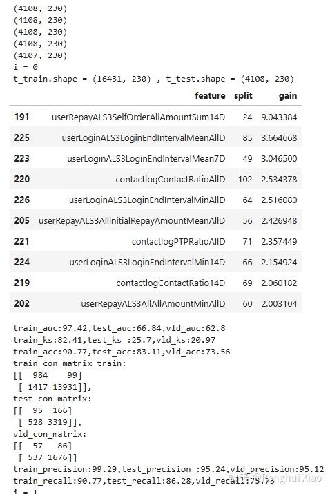
# 打印各折训练/测试/验证集指标
print("train_auc:{}, test_auc:{}, vld_auc:{}".format(...))
print("train_ks:{}, test_ks:{}, vld_ks:{}".format(...))
4.2.3 Intersection filtering
# 5次建模的 Top100 特征取交集
feature_select_df = pd.DataFrame()
for i in [0, 1, 2, 3, 4]:
    f_list = feature_name_dict[i]['feature'].to_list()
    temp_df = pd.DataFrame({'f_name': f_list, f'{i}_select': 1})
    if feature_select_df.empty:
        feature_select_df = temp_df
    else:
        feature_select_df = feature_select_df.merge(temp_df, on='f_name', how='outer')

feature_select_df = feature_select_df.fillna(0)

# 统计每个特征在5次建模中进入 Top100 的次数
feature_select_df['sum'] = feature_select_df.apply(
    lambda x: np.sum([x[f'{i}_select'] for i in [0, 1, 2, 3, 4]]), axis=1
)

# 至少4次进入 Top100 → 最终入选
select_col_list = feature_select_df[feature_select_df['sum'] >= 4]['f_name'].to_list()
Screenshots of the training process
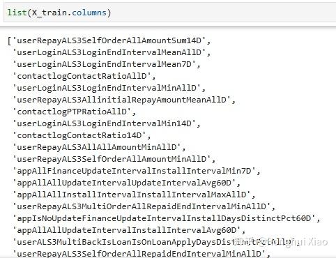
Rescreen feature set (excerpt)
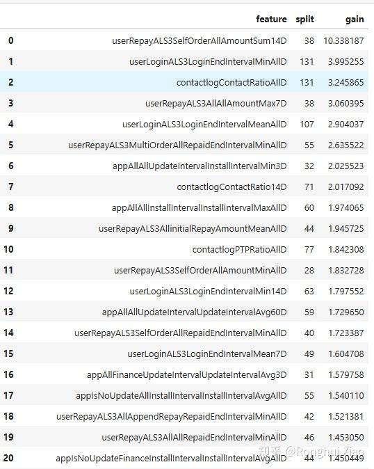
4.2.4 Final Screening: Standard LGBM Top 60 Gain Values
After two rounds of screening, a final round of screening is required to conduct a complete training on all training sets with the standard LightGBM model, and select the top 60 features with gain values as the final model version. The purpose of this step is to ensure that the features finally entered into the model have the strongest distinguishing ability on the complete data set, and it is also a re-verification and convergence of the results of the first two rounds of screening.
# 最终一次标准 LGBM 训练,取增益值 Top60 作为最终特征集
model_train2 = lgb.LGBMClassifier(is_unbalance=True)
choose_model = model_train2
choose_model.fit(X_train, y_train)

gain = choose_model.booster_.feature_importance('gain')
fi = pd.DataFrame({
    'feature': list(X_train.columns),
    'split': choose_model.booster_.feature_importance('split'),
    'gain': 100 * gain / gain.sum()
}).sort_values('gain', ascending=False).reset_index(drop=True)

# 取前60 → 最终入选特征
top_feature = fi.head(60)
Finalized feature set (TOP20)
4.2.5 Summary of screening results
After four rounds of screening, the feature scale gradually converged from the tens of thousands to about 60 high-value features, entering the formal modeling stage:
| stage | Number of features | Screening method |
|---|---|---|
| original features | tens of thousands | — |
| After IV initial screening | Thousand level | toad selection: empty=0.6, iv=0.05, corr=0.8 |
| After re-screening the gain value stability | ~82 | 5 times of random modeling × Top100 × intersection (sum ≥ 4) |
| After the final Top60 screening | ~60 | Standard LGBM gain value sorting takes the top 60 |
These approximately 60 features have gone through four rounds of screening (null value processing → IV preliminary screening → stability re-screening → LGBM Top60). They are highly robust features converged layer by layer from the tens of thousands of feature pools. They have strong distinguishing capabilities and are an important basis for the model to reach AUC 69 in long account aging scenarios.
Chapter 5: LightGBM model construction and training
5.0 LightGBM model introduction, important parameters and evaluation criteria
5.0.1 LightGBM selection background
LightGBM (Light Gradient Boosting Machine) is an efficient ensemble learning algorithm based on gradient boosting decision tree (GBDT). Compared with traditional GBDT, LightGBM adopts Histogram and Leaf-wise growth strategies, which greatly improves the training speed while maintaining good prediction accuracy. It is widely used in risk control models in the industry.
Three core reasons to choose LightGBM:
- Sparse data friendly: It has high efficiency in processing high-dimensional sparse features and is suitable for the scenario of this project with a large number of null features;
- Interpretability: The feature gain value (gain) and the number of splits (split) can be output to facilitate the analysis of feature importance;
- Fast training speed: Compared with XGBoost, LightGBM has an order of magnitude improvement in training speed in scenarios with large data volumes.
5.0.2 Important parameter description
The key parameters and functions involved in the training of this model are as follows:
| parameter | meaning | The best value of this project |
|---|---|---|
boosting_type |
Promotion method, fixed to gbdt | 'gbdt' |
objective |
objective function | 'Binary' |
learning_rate |
Learning rate, controls the step size of each iteration | 0.01 |
n_estimators |
The number of iteration rounds, the total number of trees built | 300 |
max_depth |
The maximum depth of a single tree, limiting model complexity to prevent overfitting | 2 |
num_leaves |
Number of leaf nodes, combined with max_depth to control model complexity | 3 |
min_child_samples |
The minimum number of samples for leaf nodes to avoid a few samples dominating the split | 20 |
min_child_weight |
Minimum weight of leaf nodes | 0.001 |
min_split_gain |
split minimum gain threshold | 0 |
reg_alpha |
L1 regularization coefficient, which shrinks some feature weights to 0 | 0.03 |
reg_lambda |
L2 regularization coefficient makes the feature weights overall smooth | 0.01 |
subsample |
row sampling ratio | 1 |
subsample_for_bin |
Number of sampled rows when building histogram | 200000 |
subsample_freq |
subsampling frequency | 12 |
colsample_bytree |
Column sampling ratio | 1 (0.99 during parameter search) |
is_unbalance |
Turn on sample imbalance processing | True |
max_bin |
Number of bins, number of buckets for eigenvalue bins | 900 |
importance_type |
Feature importance type | 'split' |
silent |
Whether to train silently | True |
5.0.3 Parameter training method
The hyperparameter training of this project is not a one-time black box search, but a combination of enumeration method + cross-validation + GridSearchCV + multi-index sorting combined with business goals and overfitting control requirements to gradually converge to the final parameters.
Specifically, the following methods are used:
- Enumeration method (Manual Enumeration): Traverse parameters such as learning rate, iteration rounds, regularization coefficients, and minimum number of samples group by group according to the preset range. The advantage is that the search path is clear and it is easy to control the range based on business experience;
- LightGBM native cross-validation
lgb.cv: In the first round of parameter adjustment, 5-fold cross-validation is performed on differentlearning_rate × n_estimatorscombinations, and the generalization effects of different combinations are compared with the mean CV AUC; - GridSearchCV Grid Search: In the second round of parameter adjustment, perform standard grid search on
max_depthandnum_leaves, automatically traverse the parameter combinations and return the optimal 50% CV AUC result; - Multi-indicator manual sorting: In the third round of parameter adjustment, we not only look at a single AUC, but also calculate the AUC/KS of the training set, test set, and validation set, as well as stability indicators such as
diff_ks,diff_auc, andcur_std, and then select the optimal parameter combination according to the business goals.
The core idea of this step-by-step training method is: first use cross-validation to determine the general direction parameters, then use grid search to converge the tree structure, and finally use multi-index ranking to control the risk of over-fitting, thus taking into account model effect, stability and interpretability.
5.0.4 Model training process
拿到 60 个最有特征
        │
        ▼
┌──────────────────────────────┐
│  第一步:学习率与轮数枚举       │
└──────────────────────────────┘
        │
        ▼
┌──────────────────────────────┐
│  第二步:max_depth 与          │
│  num_leaves 枚举              │
└──────────────────────────────┘
        │
        ▼
┌──────────────────────────────┐
│  第三步:L1/L2 正则化与        │
│  最小样本数枚举               │
└──────────────────────────────┘
        │
        ▼
┌──────────────────────────────┐
│  最优模型参数                 │
└──────────────────────────────┘
5.0.5 Model Evaluation Criteria
This model uses four core evaluation indicators:
AUC (Area Under ROC Curve)
The area under the ROC curve reflects the model’s ability to sort positive and negative samples. Defined as:
AUC = ∫₀¹ TPR(FPR⁻¹(x)) dx
Equivalent calculation method: Among all pairs of positive and negative samples, the model scores the positive samples higher than the proportion of negative samples.
AUC = Σᵢ Σⱼ 1[Pᵢ > Pⱼ] / (n₊ × n₋)
(where n₊ is the number of positive samples, n₋ is the number of negative samples, and 1[·] is the indicator function)
Industry standard: AUC > 65 means the model is effective, and AUC > 70 means it is good.
KS (Kolmogorov-Smirnov)
Measuring the maximum difference in the scoring distribution between good and bad samples, defined as:
**KS = maxₜ | TPR(t) − FPR(t) | **
That is, the maximum vertical distance between TPR and FPR on the ROC curve. The higher the KS, the stronger the discrimination.
Industry standard: KS > 30 is effective, KS > 40 is good.
Precision
The proportion of orders predicted as positive samples by the model actually belong to the positive sample category. Its meaning depends on which class is set as the positive class when modeling:
Precision = TP / (TP + FP)
Recall
The proportion of actual positive samples successfully predicted by the model:
Recall = TP / (TP + FN)
5.1 The first version of the model and overfitting problem
Use the 46 features filtered for stability to build a baseline LightGBM model, turn on sample imbalance processing is_unbalance=True, and the evaluation results after direct training are as follows:
train_auc: 99.98  |  test_auc: 64.54  |  vld_auc: 59.00
train_ks:  99.20  |  test_ks:  24.54  |  vld_ks:  15.90
Problem Diagnosis: The AUC of the training set is as high as 99.98, which is an almost perfect fit. However, the AUC of the test set and validation set are only around 60. The model is in a serious overfitting state - there is a huge performance gap between the training set and the validation set, indicating that the model has learned too much noise on the training data and does not have the ability to generalize.
5.2 Hyperparameter tuning method
To address the over-fitting problem, the enumeration method + cross-validation strategy is used to systematically tune all key parameters in three steps.
5.2.1 Step One: Learning Rate and Round Enumeration
Through 5-fold cross-validation, 7 combinations of learning rates × 3 n_estimators are enumerated (21 groups in total), and the optimal CV AUC mean is used as the criterion:
lr_dict = dict()
for rate in [0.01, 0.03, 0.06, 0.1, 0.3, 0.6, 1]:
    for num_boost_round in [100, 300, 600]:
        params = {
            'boosting_type': 'gbdt',
            'objective': 'Binary',
            'learning_rate': rate,
            'is_unbalance': True
        }
        data_train = lgb.Dataset(X_train_, y_train_, silent=True)
        cv_results = lgb.cv(
            params, data_train,
            num_boost_round=num_boost_round,
            early_stopping_rounds=int(num_boost_round / 2),
            nfold=5, verbose_eval=False,
            seed=3432141,
            metrics='auc', show_stdv=False
        )
        lr_dict[f"{rate}_{num_boost_round}"] = (
            cv_results['auc-mean'][-1],
            len(cv_results['auc-mean'])
        )
Summary of CV results (sorted by mean AUC):
| learning rate | Number of rounds | CV_AUC |
|---|---|---|
| 0.01 | 600 | 0.7170 |
| 0.01 | 300 | 0.7170 |
| 0.01 | 100 | 0.7170 |
| 0.03 | 600 | 0.7030 |
| 0.06 | 600 | 0.6741 |
| 0.10 | 600 | 0.6529 |
| … | … | … |
Best Choice: learning_rate=0.01, n_estimators=300
Selection criteria: Taking the 5-fold cross-validation CV AUC mean (auc-mean[-1]) as the ranking index, the lower the learning rate, the higher the AUC, and 0.01 is optimal; at the same learning rate, the AUC of 300 rounds and 600 rounds are the same (both reach 0.7170), and 300 rounds are selected for training efficiency considerations.
5.2.2 Step 2: max_depth and num_leaves enumeration
After determining the learning rate and number of epochs, use GridSearchCV to enumerate the combinations of max_depth (24) and num_leaves (37 step size 2) (9 groups in total):
model_lgb = lgb.LGBMClassifier(
    boosting_type='gbdt',
    colsample_bytree=0.99,
    importance_type='split',
    learning_rate=best_learning_rate,
    n_estimators=best_n_estimators,
    n_jobs=n_jobs,
    subsample=0.99,
    is_unbalance=True
)

params_test1 = {
    'max_depth': range(2, 5, 1),
    'num_leaves': range(3, 8, 2)
}

gsearch1 = GridSearchCV(
    estimator=model_lgb,
    param_grid=params_test1,
    scoring='roc_auc',
    cv=5, verbose=1
)
gsearch1.fit(X_train_, y_train_)

best_max_depth = gsearch1.best_params_['max_depth']
best_num_leaves = gsearch1.best_params_['num_leaves']
best_score_ = gsearch1.best_score_

print('best_learning_rate:{} best_n_estimators:{} best_num_leaves:{} best_max_depth:{}'.format(
    best_learning_rate, best_n_estimators, best_num_leaves, best_max_depth
))
best_score_
Optimal results: max_depth=2, num_leaves=3, best_score_=0.7368 (50% off CV AUC mean of the best combination of GridSearchCV)
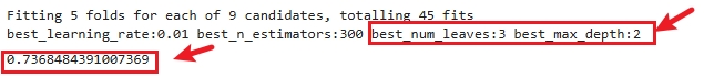
Selection criteria: scoring='roc_auc' (with ROC AUC as the scoring index), cv=5 (5-fold cross-validation), GridSearchCV takes the group with the highest average CV AUC among 9 groups of parameter combinations as the optimal solution. Extremely shallow tree depth (depth=2) is the core factor in controlling overfitting.
5.2.3 Step 3: L1/L2 regularization and minimum sample number enumeration
Finally, the regularization coefficient and the minimum number of samples of leaf nodes are enumerated (dynamic calculation) to further control the model complexity:
# 动态计算 min_child_samples 搜索范围
minsample_list = [20, 200]
minsample_list.extend(list(range(
    int(X_train.shape[0] * 0.1),
    int(X_train.shape[0] * 0.5),
    int(X_train.shape[0] * 0.05)
)))
Enumerate reg_alpha (7 types) × reg_lambda (7 types) × minsample (N types) × colsample_bytree (fixed 1 type) × subsample (fixed 1 type), and calculate three sets of indicators (training set/test set/validation set) for each set of parameters:
train_dict = dict()

for alpha in [0.001, 0.01, 0.03, 0.08, 0.3, 0.5, 1]:
    for _lambda in [0.001, 0.01, 0.03, 0.08, 0.3, 0.5, 1]:
        for minsample in minsample_list:
            for colsample in [1]:
                for subsample in [1]:
                    model_train1 = LGBMClassifier(
                        boosting_type='gbdt', class_weight=None,
                        colsample_bytree=colsample,
                        importance_type='split',
                        learning_rate=best_learning_rate,
                        max_depth=best_max_depth,
                        max_bin=900,
                        min_child_samples=minsample,
                        min_child_weight=0.001,
                        min_split_gain=0,
                        n_estimators=best_n_estimators,
                        n_jobs=n_jobs,
                        num_leaves=best_num_leaves,
                        objective=None,
                        reg_alpha=alpha,
                        reg_lambda=_lambda,
                        silent=True,
                        subsample=subsample,
                        subsample_for_bin=200000,
                        subsample_freq=12,
                        is_unbalance=True
                    )

                    choose_model = model_train1
                    choose_model.fit(X_train_, y_train_)

                    # 三集评估:训练集 / 测试集 / 验证集
                    y_pred_prob_train = choose_model.predict_proba(X_train_)[:, 1]
                    y_pred_prob_test = choose_model.predict_proba(X_test_)[:, 1]
                    y_pred_prob_vld = choose_model.predict_proba(X_vld_)[:, 1]

                    ks_train = cal_ks(yprob=y_pred_prob_train, ytrue=y_train_.values)
                    ks_test = cal_ks(yprob=y_pred_prob_test, ytrue=y_test_.values)
                    ks_vld = cal_ks(yprob=y_pred_prob_vld, ytrue=y_vld_.values)

                    auc_train = roc_auc_score(y_score=y_pred_prob_train, y_true=y_train_.values)
                    auc_test = roc_auc_score(y_score=y_pred_prob_test, y_true=y_test_.values)
                    auc_vld = roc_auc_score(y_score=y_pred_prob_vld, y_true=y_vld_.values)

                    diff_ks = abs(ks_train - ks_vld)
                    diff_auc = abs(auc_train - auc_vld)
                    cur_std = np.std(np.array([ks_test, ks_vld, auc_test, auc_vld]))

                    key = f'{alpha}_{_lambda}_{minsample}_{colsample}_{subsample}'
                    temp_dict = {
                        'ks_train': ks_train, 'ks_test': ks_test, 'ks_vld': ks_vld,
                        'auc_train': auc_train, 'auc_test': auc_test, 'auc_vld': auc_vld,
                        'diff_ks': diff_ks, 'diff_auc': diff_auc, 'cur_std': cur_std
                    }
                    train_dict[key] = temp_dict
Finally, the optimal combination is determined through the following rules:
train_df = pd.DataFrame().from_dict(train_dict, orient='index')
train_df.sort_values(by='ks_vld', ascending=False).head(20)
In the sorting results, ks_vld and auc_vld of the Top 5 combinations are basically the same, and all fall near min_child_samples=20, indicating that controlling the minimum number of leaf samples is the most critical constraint in this round of parameter tuning. Finally, the combination ranked first is selected:
Training result legend
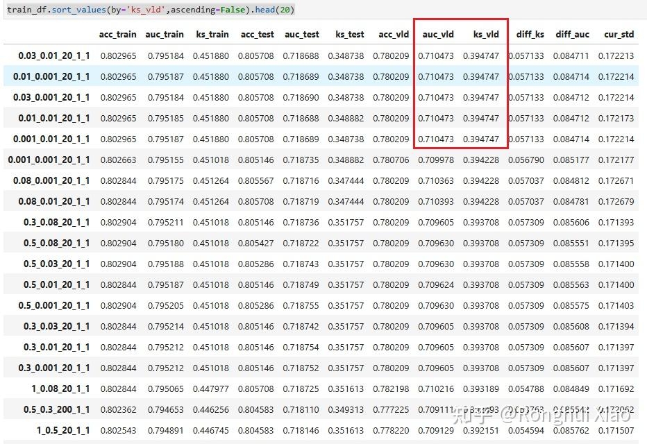
Best choice: reg_alpha=0.03, reg_lambda=0.01, min_child_samples=20
The key indicators corresponding to this combination are: auc_train=0.7952, auc_test=0.7187, auc_vld=0.7105, ks_train=0.4519, ks_test=0.3487, ks_vld=0.3947, diff_ks=0.0571. This shows that it not only has the highest KS in the validation set, but also has a relatively balanced performance among the three episodes.
Selection criteria: Taking ks_vld (validation set KS) as the core sorting index, take the Top 20 in descending order, supplemented by diff_ks (difference between training set/validation set KS), diff_auc (difference between training set/validation set AUC), cur_std (four indicators comprehensive stability) comprehensive evaluation. ks_vld directly reflects the model’s ranking and discrimination ability on unseen data. The difference and stability indicators are used to ensure that the selected parameters have good generalization capabilities and are not optimal by chance.
Optimal parameter combination:
| parameter | optimal value | source |
|---|---|---|
learning_rate |
0.01 | 5.2.1 Optimal |
n_estimators |
300 | 5.2.1 Optimal |
max_depth |
2 | 5.2.2 GridSearchCV optimal |
num_leaves |
3 | 5.2.2 GridSearchCV optimal |
reg_alpha(L1) |
0.03 | 5.2.3 ks_vld optimal |
reg_lambda (L2) |
0.01 | 5.2.3 ks_vld optimal |
min_child_samples |
20 | 5.2.3 ks_vld optimal |
Summary of overall selection criteria for three-step tuning:
| step | Tuning goals | Number of parameter combinations | Judgment criteria |
|---|---|---|---|
| 5.2.1 Learning rate + number of rounds | 7×3 = 21 groups | 5-fold cross-validation CV AUC has the highest mean value | |
| 5.2.2 max_depth+num_leaves | 3×3 = 9 groups | GridSearchCV 50% off CV AUC with the highest mean value | |
| 5.2.3 Regularization + minimum number of samples | 7×7×N group | ks_vld verification set KS is the highest, supplemented by diff_ks/diff_auc/cur_std comprehensive evaluation |
5.3 Final model effect
After applying the optimal parameter combination, the model evaluation results are as follows:
| Dataset | AUC | KS | Precision | Recall |
|---|---|---|---|---|
| train | 79.52 | 45.19 | 6.47% | 59.02% |
| test | 71.87 | 34.87 | 5.71% | 50.32% |
| vld (validation set) | 69.05 | 39.47 | 10.77% | 57.65% |
Comparison before and after optimization:
| stage | train_auc | test_auc | vld_auc | train_ks | test_ks | vld_ks | Precision | Recall |
|---|---|---|---|---|---|---|---|---|
| Before optimization (serious overfitting) | 99.98 | 64.54 | 59.00 | 99.20 | 24.54 | 15.90 | — | — |
| After optimization (after parameter adjustment) | 79.52 | 71.87 | 69.05 | 45.19 | 34.87 | 39.47 | 10.77% | 57.65% |
After optimization:
- The AUC gap between the training set and the validation set is reduced from 40.98 to 10.47, and the over-fitting problem is significantly improved;
- The verification set AUC increased from 59.00 to 69.05, and KS increased from 15.90 to 39.47, reaching the industry’s effective standard of AUC 65+ / KS 30+;
- The model has practical business application value.
5.4 Core means to solve overfitting
| means | effect |
|---|---|
max_depth=2 |
Limit the maximum depth of a single tree to prevent over-fitting from being too deep. |
num_leaves=3 |
Limit the number of leaf nodes and use depth to control model complexity |
reg_alpha=0.03 (L1) |
L1 regularization, shrinking some feature weights to 0 |
reg_lambda=0.01 (L2) |
L2 regularization makes the feature weights overall smooth |
min_child_samples=20 |
Limit the minimum number of samples of leaf nodes to avoid a few samples dominating the split |
learning_rate=0.01 + n_estimators=300 |
A low learning rate combined with a sufficient number of rounds ensures that the model fully converges without overfitting. |
Chapter 6: Model Validation and Evaluation
6.1 Score distribution verification
Convert the default probability output by the model into a standard credit score (0 to 1000 points) through logistic transformation, and test whether its distribution on the verification set is reasonable and whether it exhibits the expected monotonic distinguishing ability.
Validation set score distribution:
| Fractional section | goods (repayment) | bads (unpaid) | Repayment ratio |
|---|---|---|---|
| 414–465 | 2 | 183 | 1.08% |
| 466–475 | 4 | 180 | 2.17% |
| 476–482 | 5 | 228 | 2.15% |
| 483–490 | 4 | 182 | 2.15% |
| 491–498 | 8 | 206 | 3.74% |
| 499–505 | 5 | 188 | 2.59% |
| 506–515 | 5 | 208 | 2.35% |
| 516–530 | 3 | 192 | 1.54% |
| 531–551 | 19 | 186 | 9.27% |
| 552–618 | 30 | 173 | 14.78% |
Hierarchical data normal distribution plot

Distribution Characteristic Analysis:
- Good monotonicity: The higher the score, the more repayment samples (goods) and the fewer non-repayment samples (bads), and the score has strong monotonic discrimination ability;
- Continuous smooth distribution: The number of people in each segment is basically stable between 180 and 233, with no cliff-like decline or abnormal peaks, and the curve is smooth;
- Business explainable: The repayment probability of high-segmented users is significantly higher than that of low-segmented users, and the scores can be directly mapped to the collection priority.
6.2 Cross-time stability verification
In order to ensure the consistency of the model’s performance in different time periods and avoid the degradation of the model’s generalization ability due to time factors, the validation set was split according to time windows and evaluated separately.
Conclusion: The overall fluctuations of AUC and KS indicators in each time window are within the acceptable range, and there is no obvious time attenuation phenomenon. The performance of the model in different time periods is stable, and it has the conditions for continuous investment in business applications.
Chapter 7: Business Effect and ROI Analysis
7.1 ROI improvement curve
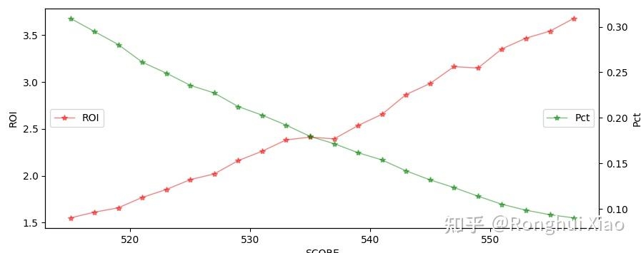
After the model is launched, the business side selects orders from high to low according to the model score for collection. The corresponding relationship between the proportion of detected orders and the labor efficiency ratio (ROI) is as follows:
| Score Pct (score percentile) | Proportion of checkout orders (%) | ROI |
|---|---|---|
| 0 | 31.38 | 1.52 |
| 6 | 22.23 | 2.01 |
| 10 | 17.90 | 2.40 |
| 13 | 14.97 | 2.54 |
| 15 | 13.23 | 2.92 |
| 20 | 8.85 | 3.64 |
| twenty four | 6.71 | 4.62 |
| 28 | 5.27 | 5.59 |
Note: Score Pct = 0 represents the lowest segment (covering the most orders), Score Pct = 28 represents the highest segment (covering the fewest orders).
Proportion of checkout orders and manpower energy efficiency ratio
7.2 ROI compliance analysis
- When Score Pct = 6 (approximately 22% of orders are checked out), the ROI breaks through 2.0, exceeding the ROI > 2.0 target proposed by the business;
- When Score Pct = 13 (approximately 17% of orders are checked out), the ROI reaches 2.54, and the labor investment is reduced by more than half, but the ROI is still maintained above 2.5;
- When Score Pct = 15 (approximately 13% of orders are detected), the ROI reaches 2.92, which is nearly twice the ROI of 1.5 in the reminder mode;
- When Score Pct = 20 (approximately 9% of orders are checked out), the ROI reaches 3.64. With less than one manpower invested, the ROI more than triples.
7.3 Summary of business value
| index | reminder mode | Model detection (about Top 20%) |
|---|---|---|
| Human input | Full reminder | About 20% of orders |
| ROI | 1.0~1.5, mean 1.1 | ~2.12 |
| Target ROI > 2.0 | Not up to standard | Overachieved |
After the model was launched, the business side actually calculated that the ROI reached 2.12, exceeding the set target (> 2.0), significantly saving labor costs and maximizing collection income.
Chapter 8: Prediction Model Optimization - Auxiliary Model Online
8.1 Online background
After the LGBM prediction model was launched online, it has completed the core goals set by the business department: sorting long-aging orders through the model, screening out high-value orders and investing in manual collection. While significantly reducing labor investment, it has achieved ROI improvement and verified that the path of “model detection + human focus” is established in business.
However, in the actual implementation process, a natural limitation of the prediction model has gradually been exposed: when the main model is scoring, it can only use the features that have settled before the stage enters the market. This means that the information the model relies on is essentially a historical portrait of the user before entering the current stage, and cannot reflect the user’s new changes within the stage in a timely manner.
From a modeling perspective, this approach is reasonable, because it ensures the strict separation of tag time points and feature time points, and avoids information crossing; but from a business perspective, this also brings about a practical problem: some orders are not detected during the initial screening of the main model, which does not mean that they will never have recovery value in the future. If users have new positive behaviors within a stage, these behaviors themselves mean that their repayment willingness, fund status, or processing priorities may have changed.
Therefore, the focus of this round of optimization is not to redo the main model, but to add a layer of dynamic recognition capabilities to the main model.
8.2 Boundaries of the main model
The core capability of the main model is to sort orders in one go based on the historical behavior before the stage enters the market. This method is suitable for solving the problem of “which orders are more worthy of prioritizing manpower investment at a fixed point in time”, but it is difficult to answer another more dynamic question:
Do some orders that were not worth recalling in the first place regain their recall value due to changes in user behavior as the stages progress?
This is exactly where the boundaries of the main model lie.
Specifically, there are two main limitations:
First, features have natural hysteresis.
The model uses pre-order features, and long-aging orders themselves are already a scenario with a strong time lag. After entering this stage, the user’s behavior may have changed significantly, such as logging in to the APP again, checking bills, repaying other debt-sharing platform orders, etc. These signals do not exist when the main model scores, and therefore cannot be used by the main model.
Second, the main model is a one-time filtering logic and does not have the ability to dynamically update.
The main model is more like a static sorter: at a fixed point in time, orders are divided into two categories: “priority reminder” and “suspension reminder”. But real business is not static, and users’ behavior will continue to change within stages. If you still insist on only looking at the initial scoring results, you may miss some “subsequent strengthening” orders.
In other words, the main model solves the problem of “who urges first”, but does not completely solve the problem of “who deserves to be urged later”.
8.3 Business Insight: Behavior within the stage may bring new recovery value
After further communication with the business department around this issue, we came to a very critical empirical judgment:
Some of the user’s behaviors during the stage may themselves constitute a signal that “it is worth urging again”.
These behaviors may not necessarily be reflected in the static scoring of the main model, but they have obvious reference value in actual collection experience. Typical include:
- User logs in to the APP again: It means that the user is still actively contacting the platform, at least not completely lost contact, and may have behavioral motivations such as checking bills, paying attention to credit limits, preparing to deal with arrears, etc.;
- User repays other mutual debt orders: It shows that the user has recent capital flow, and it also shows that he is not completely incapable of repaying, but is prioritizing between different debts;
- Active behaviors of users in other stages: such as revisiting key pages, re-triggering certain actions, etc., may also mean that their status has changed.
The nature of these signals is very similar to the “timing” logic in quantitative investment. The main model is more like an “initial stock selection model”, responsible for screening out a batch of high-potential orders at the initial time point; while the intra-stage behavioral signals are more like “timing signals”, used to determine whether certain orders that did not originally enter the candidate pool have reappeared in the subsequent time points with intervention value.
Therefore, the one-time scoring of the main model alone is not enough. A supplementary mechanism is also needed to conduct secondary identification of orders with new signals within the stage. This is the starting point for the launch of the auxiliary model.
8.4 Ideas for launching auxiliary models
Based on the above background, this round of prediction model optimization is not to overthrow the main model, but to add a layer of “order recovery strategy” based on the main model’s completion of business goals.
The core idea of this strategy is:
-
The main model continues to assume the responsibility of the main screen The main model still completes the first round of sorting at the starting point of the stage, and selects the high-value orders that deserve priority for manual collection.
-
Continuous observation of orders that have not been checked out by the main model For those orders that do not enter the collection list for the first time, they are not directly regarded as permanently low value, but their behavior changes are continued to be observed within the stage.
-
Trigger retrieval based on new behavioral signals Once an order shows certain key behaviors within a stage, such as logging in, repaying other debt orders, becoming active again, etc., it will be identified as an object whose “status may change” and enter the scope of secondary evaluation.
-
Dynamic supplementary recognition is undertaken by the auxiliary model Let the main model be responsible for the “initial checkout” and the auxiliary model be responsible for the “midway recovery” to jointly form a collection screening system that is closer to the real business rhythm.
In other words, the goal of the auxiliary model is not to replace the main model, but to supplement the blind spots of the main model: Those orders whose prices were not strong enough at the initial stage but became strong as the stage progresses will be brought back into the collection scope.
8.5 Final screening results of auxiliary models
After multiple rounds of business discussions and signal verification, the auxiliary model finally retained the three most effective, easiest to explain, and most suitable for implementation:
-
User logs in during the stage The login behavior shows that the user is still actively contacting the platform and has not completely lost contact. For long-aging orders, this kind of behavior often means that users begin to pay attention to bills, quotas or historical orders again, which has a certain value for subsequent contact.
-
The user repaid other orders This signal indicates that users are not completely deprived of funds in the near future, but are prioritizing allocations among different debts. Now that the user has started processing other orders, it means that the current order may be further recalled.
-
The order itself is a partial repayment order Partial repayment shows that the user does not completely refuse to perform the contract, but has shown a certain degree of willingness to repay. For this type of order, subsequent investment in collection resources is usually more valuable than an order with no repayment action at all.
What these three features have in common is that they are not static images before entering the market, but dynamic behavioral signals that appear during the stage, so they are very suitable as the core retrieval conditions of the auxiliary model.
8.6 Auxiliary model online effect
After the auxiliary model was launched, based on the original detection results of the main model, further supplementary identification of edge high-value orders was achieved. The final effect is as follows:
- Check out about 10% more orders
- The repayment rate for checkout orders increased from 10% to 15.8%
- Overall ROI improved to 2.5
This shows that although the auxiliary model does not replace the main model, it successfully improves the quality of the detection results through the supplementary identification of dynamic signals within the stage, and further enhances the output efficiency of collection resources.
8.7 Business value
If the value of the main model lies in “improving the efficiency of first-round detection,” then the value of the auxiliary model lies in “reducing the opportunity loss caused by missed detections.”
It can bring at least three benefits:
First, improve the coverage of high-value orders.
Some of the orders that were not originally checked out will regain their recall value due to changes in behavior during the stage. Through the clawback strategy, the effective coverage can be expanded and the probability of missing potentially recallable orders can be reduced.
Second, make the collection strategy closer to the real business process.
Collection is not a one-time action, but an ongoing process. After the auxiliary model incorporates the behavior within the stage into the judgment logic, the entire strategy is upgraded from static decision-making to dynamic decision-making, which is more in line with business reality.
Third, lay the foundation for subsequent more refined strategies.
Once the retrieval logic is verified to be effective, it can continue to evolve into a more systematic dynamic strategy system in the future, such as designing different retrieval priorities according to different signal strengths, or further productizing and regularizing retrieval signals to form standard operating actions.
8.8 Summary
The LGBM prediction model has proven that screening high-value long-aging orders through the model can significantly improve collection ROI, and the business path is established.
The significance of this round of prediction model optimization is to further acknowledge and utilize a fact: The value of an order is not static. The user’s new behavior during the stage may make the order that was not checked out regain the recall value.
Therefore, the essence of this launch is not to retrain a completely different main model, but to superimpose a layer of dynamic recovery logic based on behavioral signals within the stage on the basis of the original static detection capabilities, so that the collection strategy can be upgraded from “only looking at the starting point” to “continuous observation and dynamic correction”.
This is also a key step from “single point prediction” to “prediction + dynamic supplementary identification”.
Chapter 9: Methodological Precipitation and Reflection
9.1 Data level
Feature hysteresis problems and solutions
The progress of the project has not been smooth sailing. The verification set AUC of the first version of the model is only 50~55, which is far lower than the industry’s passing line of 65. The model has almost no actual ranking ability.
After investigation, it was found that the root cause of the problem lies in: long-aged users have passed a long time since their initial application, and there is a large lag in the user information stored in the feature library. Early static features cannot effectively distinguish between repaying and non-repaying users.
The solution idea in the first stage is to introduce more recent behavior characteristics (login behavior in the past 3 days/7 days, recent repayment records, etc.) into the main model, and refine the time window with smaller granularity, using recent information to make up for the lag of historical information. The final verification set AUC increased from 55 to 69, reaching the industry’s effective standard.
But this project also further verified that even if the main model has been optimized, the long aging scenario still naturally has the problem of “characteristics continue to change after the payment is received”. It is precisely because of this that it is necessary to add a layer of auxiliary models in addition to the main model in the future to dynamically identify and retrieve new behavioral signals during the stage.
9.2 Algorithm level
Overfitting prevention and control experience
The train_auc of the first version of the LGBM prediction model is as high as 99.98, but the test_auc is only 59.55, which is seriously overfitting. Finally, it was successfully solved by the following means:
- Tree depth control:
max_depth=2,num_leaves=3, extremely shallow tree depth is the core of controlling over-fitting; - Regularization:
reg_alpha=0.03(L1) andreg_lambda=0.01(L2) are used together to smooth the feature weights; - Minimum sample number limit:
min_child_samples=20, to avoid a small number of samples dominating the split; - Low learning rate:
learning_rate=0.01with 300 rounds to prevent over-fitting while fully training.
Core lesson: In sparse scenarios, model complexity control is more important than the model itself; stabilizing the main model first, and then superimposing auxiliary strategies is far more effective than putting all problems on a single model at the beginning.
9.3 Business level
Models serve business, not show off skills
The most important business gain from this project is: the value of the model does not lie in pursuing the highest AUC, but in achieving business goals with the lowest labor cost.
The ROI of the reminder mode is only 1.5. The core reason is not that the model is not accurate enough, but that the full amount of reminders leads to a waste of manpower. This project first uses the LGBM prediction model to screen out the Top 20% of high-value orders, and the ROI is increased to 2.12; then the auxiliary model is used to dynamically recover orders that have become stronger again during the stage, and finally the ROI is increased to above 2.5. The dismantling of business goals is more important than the improvement of model indicators.
More importantly, this project illustrates a very practical methodology:
- The main model solves the first round of detection problems
- Auxiliary model solves dynamic supplementation problem
In other words, business strategies may not always be “one model solves all problems.” In many cases, a more effective way is to separate the static prediction and dynamic identification, design them separately, and then combine them for implementation.
9.4 Directions for improvement
- Online learning: The current main model is still trained offline, and incremental updates can be explored to adapt to user behavior drift;
- Productization of auxiliary model rules: Precipitate signals such as login within the stage, repayment of other orders, and partial repayment into a standardized recovery engine to reduce manual maintenance costs;
- Cross-product line migration: This combined framework of “main model detection + auxiliary model recovery” can be reused in post-loan risk control scenarios of other credit product lines;
- More fine-grained stratification: Upgrade from two categories to multiple categories, and implement differentiated collection strategies for high/medium/low-risk users.