
The Research on the Short Memory Principle of Fractional-Order Systems
This article is adapted from my 2021 thesis titled Short Memory Principle for Fractional-Order Systems. It documents my research process around this topic and the insights I developed.
My initial interest in fractional-order systems did not come from finding the definitions novel, but from their distinctive modeling approach: the current state of a system is not determined solely by the present moment—it continuously depends on its entire historical trajectory. This memory property is precisely why fractional-order models often outperform ordinary integer-order models in areas like viscoelastic materials, anomalous diffusion, and control systems.
The core problem this thesis tackles is clear: while fractional-order systems better capture memory-dependent dynamics, they are computationally much harder. Terms like the fractional integral $\int_0^t (t-\tau)^{-\alpha}f(\tau)d\tau$ require discretizing and summing over the entire history from 0 to $t$. As time grows, so does the number of history terms—each step forward costs more than the last, and overall algorithmic complexity escalates rapidly.
To address this, the thesis adopts two main approaches. The first is the Predictor-Corrector Method, used to construct numerical schemes for both constant-order and variable-order fractional systems. The second is the Short Memory Principle, which truncates the full historical integral to the most recent segment of length $T$, reducing complexity from $O(N^2)$ to $O(N \cdot T/h)$. The thesis does more than just combine these two—it analyzes how well this combination balances accuracy and efficiency.
Specifically, the thesis does two things. First, it applies the predictor-corrector method systematically to constant-order and variable-order fractional systems, comparing numerical accuracy across different algorithms. Second, it introduces the short memory strategy into these algorithms, investigating how truncation affects error, how much computation time is saved, and how to choose the optimal memory length $T$.
The most valuable conclusion I eventually arrived at—and the reason I wanted to write this up separately—is this: the short memory method is not merely an “engineering trick for speed.” There is a deeper quantitative question underneath: what exactly is the relationship between the fractional order $\alpha$ and the optimal memory length $T$? Through experiments on both constant-order and variable-order systems, the thesis demonstrates that short memory can effectively reduce computation cost, and that changes in $\alpha$ directly influence the choice of $T$. This is one of the central insights of the entire work.
This article largely preserves my original thought process, though the introduction lays out the overall framework first. To make the blog post more readable, it is organized as: concepts foundations → constant-order algorithms → variable-order extensions → conclusions and insights. You can think of it as answering three questions:
- Why are fractional-order systems harder to compute than integer-order systems?
- Why can the short memory principle significantly speed up computation?
- To what extent can this truncation strategy work in both constant-order and variable-order settings?
1. Fundamentals of Fractional-Order Systems
This chapter introduces the core concepts that will be used throughout the rest of the article. The most important takeaways are: how fractional derivatives differ from ordinary derivatives, why the predictor-corrector method becomes the most common numerical tool for these problems, and why the short memory principle has a chance of working.
1.1 Several Common Definitions of Fractional Calculus
Before diving into the algorithms, let us distinguish the three most common definitions of fractional calculus. These are not competing theories—they are different expressions of the same underlying mathematics in different contexts: some are better suited for numerical discretization, others for theoretical analysis, and still others for initial value problems. The definitions that the thesis actually relies on most heavily are the Caputo derivative for modeling purposes and the GL (Grönwall-Letnikov) intuition for discretization.
1. Grünwald-Letnikov (GL) Derivative
The Grünwald-Letnikov derivative is the definition most directly connected to “discrete history summation.” It is particularly important in numerical computation, because it essentially tells us: a fractional derivative does not depend only on a local neighborhood—it accumulates a whole string of past states with weights. The $\alpha$-order GL derivative is written as:
$$ D_{GL}^{\alpha}f(t) = \lim_{h \to 0} h^{-\alpha} \sum_{j=0}^{\lfloor t/h \rfloor} (-1)^j \binom{\alpha}{j} f(t-jh) $$
where the binomial coefficient $\displaystyle \binom{\alpha}{j} = \frac{\alpha(\alpha-1)(\alpha-2)\cdots(\alpha-j+1)}{j!}$. From this form, the “memory” characteristic of fractional systems is already visible: the derivative at the current time absorbs an entire history of past states, rather than depending only on a local neighborhood like an integer-order derivative.
2. Riemann-Liouville Integral
The Riemann-Liouville fractional integral is defined as:
$$ I_{RL}^{\alpha}f(t) = \frac{1}{\Gamma(\alpha)} \int_0^t (t-\tau)^{\alpha-1} f(\tau) d\tau $$
where $\Gamma$ is the gamma function. The RL integral can define fractional order for any $\alpha > 0$ and exhibits derivative-like properties. It is commonly used in theoretical analysis and analytical solutions.
3. Caputo Derivative
The Caputo derivative is another widely used fractional definition:
$$ {}^C D_t^{\alpha}f(t) = \frac{1}{\Gamma(1-\alpha)} \int_0^t (t-\tau)^{-\alpha} f’(\tau) d\tau $$
When handling initial value problems, the Caputo derivative is more convenient, because its initial conditions are consistent with those of ordinary differential equations—no additional RL-type initial conditions are needed. This is why, when building numerical schemes later, I naturally take the Caputo form as the starting point.
4. Comparison of the Three Definitions
| Definition | Typical Use Case | Initial Condition Handling |
|---|---|---|
| GL Derivative | Numerical discretization | Requires additional treatment |
| RL Integral/Derivative | Theoretical analysis, analytical solutions | Needs RL initial conditions |
| Caputo Derivative | Engineering applications, initial value problems | Same as integer-order equations |
1.2 The Predictor-Corrector Method
Before discussing whether history can be truncated, we need to answer a more fundamental question: how to stably solve the original equation numerically. The Predictor-Corrector Method is conceptually straightforward: first use a cheaper formula for a Predictor step (P), then substitute the predicted value into a more accurate Corrector step (C). It balances implementation difficulty, computational efficiency, and accuracy, which is why it is so common in fractional numerical computation.
For the Caputo fractional differential equation $D^{\alpha}y(t) = f(t, y(t)),\ y(0) = y_0$, its integral form is:
$$ y(t) = y_0 + \frac{1}{\Gamma(\alpha)} \int_0^t (t-\tau)^{\alpha-1} f(\tau, y(\tau)) d\tau $$
Discretizing this integral form yields the predictor and corrector coefficients that appear repeatedly in what follows. In essence, every seemingly complex recurrence formula in this thesis is an elaboration of this relationship. After establishing the standard form for constant-order systems, we will extend it to variable-order settings.
1.3 The Short Memory Principle
With a basic numerical framework in place, we arrive at the central question of this thesis: can the historical integral be shortened? The fractional integral $\int_0^t (t-\tau)^{-\alpha}f(\tau)d\tau$ accumulates the entire history, but when $\alpha \in (0, 1)$, the influence of more distant history is typically weaker. This raises the natural question: can we keep only the “most recent” segment of history and discard everything earlier?
The short memory principle truncates the integral history to the most recent interval of length $T$:
$$ I_{\text{short}}^{\alpha}f(t) \approx \frac{1}{\Gamma(\alpha)} \int_{t-T}^{t} (t-\tau)^{\alpha-1} f(\tau) d\tau $$
The real difficulty is not “whether to truncate,” but: how large should $T$ be, so that speedup is achieved while keeping error under control? This question—though it sounds like a parameter selection issue—is precisely the central research entry point of the entire thesis.
2. Numerical Computation for Constant-Order Fractional Systems
2.1 Basic Idea of the Predictor-Corrector Method
Before studying variable-order systems, the thesis begins with the simpler constant-order fractional system. Consider the general constant-order fractional differential equation initial value problem:
$$ {}^C D_t^\alpha y(t) = f(t, y(t)), \quad 0 < \alpha < 1, \quad y(0) = y_0 $$
From the literature, this equation is equivalent to the following Volterra integral equation:
$$ y(t) = y_0 + \frac{1}{\Gamma(\alpha)} \int_0^t (t-\tau)^{\alpha-1} f(\tau, y(\tau)) d\tau $$
The approach here is not to derive the fractional case from scratch, but to first review the familiar Adams predictor-corrector method for first-order ODEs, then extend this quadrature idea to constant-order fractional equations.
For a first-order ODE initial value problem at the undergraduate level, if a unique solution exists on the interval, the Adams predictor-corrector method can be used. Let the interval length be $T$, the number of steps be $N$, and the step size be $h = T/N$. The core idea is: first obtain a predicted value through a simple prediction formula, then substitute it into a more accurate correction formula to get a better approximation for the next step.
With this background, we return to the constant-order fractional equation. Since the integral in the formula extends from 0 to the current time—reflecting the nonlocal nature of fractional systems—we can still use the predictor-corrector quadrature idea. Take an equally spaced grid:
$$ t_k = kh, \quad k = 0, 1, \dots, n+1 $$
and denote $y_k \approx y(t_k)$. At $t_{n+1}$, the above equation becomes:
$$ y(t_{n+1}) = y_0 + \frac{1}{\Gamma(\alpha)} \int_0^{t_{n+1}} (t_{n+1} - \tau)^{\alpha-1} f(\tau, y(\tau)) d\tau $$
Partition the integral interval into subintervals:
$$ \int_0^{t_{n+1}} = \sum_{j=0}^{n} \int_{t_j}^{t_{j+1}} $$
The approximation used in the thesis applies linear interpolation to the integrand at the nodes, yielding the correction and prediction formulas. After reorganization, the predictor-corrector scheme for constant-order fractional differential equations is:
$$ y_{n+1}^{P} = y_0 + \frac{h^\alpha}{\Gamma(\alpha+1)} \sum_{j=0}^{n} b_{j,n+1} f(t_j, y_j) $$
where the prediction coefficients are:
$$ b_{j,n+1} = (n+1-j)^\alpha - (n-j)^\alpha, \qquad j = 0, 1, \dots, n $$
The correction formula is:
$$ y_{n+1} = y_0 + \frac{h^\alpha}{\Gamma(\alpha+2)} \left[ \sum_{j=0}^{n} a_{j,n+1} f(t_j, y_j) + f(t_{n+1}, y_{n+1}^{P}) \right] $$
where the correction coefficients are:
$$ a_{j,n+1} = \begin{cases} n^{\alpha+1} - (n-\alpha)(n+1)^\alpha, & j = 0, \ (n-j+2)^{\alpha+1} + (n-j)^{\alpha+1} - 2(n-j+1)^{\alpha+1}, & 1 \le j \le n, \ 1, & j = n+1. \end{cases} $$
At this point, the predictor-corrector formula for constant-order fractional differential equations is fully established. All subsequent numerical experiments are built around this scheme.
2.2 Introduction of the Short Memory Principle in Constant-Order Systems
In the original predictor-corrector formulas, all terms except the last one depend only on the current neighborhood. However, the final summation—because the integral runs from 0 to the current step—always involves the entire function history. This is precisely what the short memory principle addresses.
Truncation Idea
The approach taken in the thesis is a fixed memory length strategy. Let the preserved integral length be $T$. When the summation length exceeds this interval, we truncate the earlier history from the starting side and keep only the most recent segment of length $T$.
Denote:
$$ M = \left\lfloor \frac{T}{h} \right\rfloor $$
If the current step $n \le M$, the current integral interval has not yet exceeded the length to be preserved, so no truncation is needed—the summation still starts from 0.
If $n > M$, we discard the earlier history and keep only:
$$ j = n-M,; n-M+1,; \dots,; n $$
In this case, the prediction step is rewritten as:
$$ y_{n+1}^{P} = y_0 + \frac{h^\alpha}{\Gamma(\alpha+1)} \sum_{j=n-M}^{n} b_{j,n+1} f(t_j, y_j) $$
The correction step is rewritten as:
$$ y_{n+1} = y_0 + \frac{h^\alpha}{\Gamma(\alpha+2)} \left[ \sum_{j=n-M}^{n} a_{j,n+1} f(t_j, y_j) + f(t_{n+1}, y_{n+1}^{P}) \right] $$
In other words, once the integral interval exceeds $T$, the lower limit of the summation is no longer fixed at 0, but changes to near $n - T/h$.
Why is this justified? Two analytical perspectives are useful:
1. Analytical Method
When calculating the truncation error, given an allowable precision $E$, the integral length $T$ can theoretically be derived inversely from the corresponding error formula. The thesis shows that when the fractional order is in $[0, 1]$, a fixed memory length can reduce computation, and the chosen integral length is independent of the original total integral length. When the order exceeds this range, the fixed-length approach no longer works as easily, and selecting $T$ becomes more difficult.
2. Weight Function Image Analysis
In addition to theoretical error analysis, the thesis provides a more intuitive approach: re-examine the distributions of the prediction coefficient $b$ and correction coefficient $a$. The images show that when the step count is close to the current time, the weight function values increase significantly, while earlier history nodes have smaller weights; additionally, smaller order values lead to even smaller early weights. This indicates that for smaller orders, the system depends less on distant history, and the weight function image can serve as a guide for choosing the integral length $T$.
2.3 Algorithm
After the above analysis, the thesis organizes the predictor-corrector algorithm with short memory into a set of implementation steps:
- Input known parameters: initial conditions, step size, and full integral interval.
- Determine the preserved integral length $T$ using the weight function image.
- Compute the predicted value for the next step using the prediction formula.
- Substitute the predicted value into the correction formula to obtain the corrected value.
- When the step count is less than $T/h$, the summation starts from 0.
- When the step count exceeds $T/h$, the summation starts from $n - T/h$.
With this, the predictor-corrector algorithm with short memory is fully established. The thesis then proceeds to numerical examples for verification.
2.4 Constant-Order Examples and Error Analysis
2.4.1 Example 1
$$D_*^\alpha x(t) = \frac{\Gamma(9)}{\Gamma(9-\alpha)} t^{8-\alpha} + \frac{9}{4}\Gamma(\alpha+1) + t^8 + \frac{9}{4}t^\alpha - x(t)$$
Initial conditions: $x(0) = 0,\ x’(0) = 0$
Exact solution: $x(t) = t^8 + \frac{9}{4} t^\alpha$
This example considers $\alpha = 0.7$ and $\alpha = 1.7$, corresponding to two important intervals $(0, 1)$ and $(0, 2)$.
Interval $(0, 1)$, $\alpha = 0.7$, comparison across step sizes:
$h = 1/160$
| $t$ | Exact value $x(t)$ | Numerical solution | Absolute error | Relative error% |
|---|---|---|---|---|
| 0.1 | 0.4489 | 0.4563 | 0.0074 | 1.64 |
| 0.3 | 0.9687 | 0.9824 | 0.0136 | 1.41 |
| 0.5 | 1.3889 | 1.4064 | 0.0175 | 1.26 |
| 0.7 | 1.8105 | 1.8316 | 0.0211 | 1.16 |
| 0.9 | 2.5205 | 2.5494 | 0.0289 | 1.15 |
$h = 1/320$
| $t$ | Exact value $x(t)$ | Numerical solution | Absolute error | Relative error% |
|---|---|---|---|---|
| 0.1 | 0.4489 | 0.45343 | 0.00453 | 1.01 |
| 0.3 | 0.9687 | 0.97707 | 0.00837 | 0.86 |
| 0.5 | 1.3889 | 1.3997 | 0.01080 | 0.78 |
| 0.7 | 1.8105 | 1.8234 | 0.01290 | 0.71 |
| 0.9 | 2.5205 | 2.5382 | 0.01770 | 0.70 |
$h = 1/640$
| $t$ | Exact value $x(t)$ | Numerical solution | Absolute error | Relative error% |
|---|---|---|---|---|
| 0.1 | 0.4489 | 0.45169 | 0.00279 | 0.62 |
| 0.3 | 0.9687 | 0.97384 | 0.00514 | 0.53 |
| 0.5 | 1.3889 | 1.3955 | 0.00660 | 0.48 |
| 0.7 | 1.8105 | 1.8184 | 0.00790 | 0.44 |
| 0.9 | 2.5205 | 2.5314 | 0.01090 | 0.43 |
The tables show that for this example, the predictor-corrector method achieves high accuracy, and accuracy improves monotonically as the step size decreases.
Interval $(0, 2)$, $\alpha = 1.7$, $h = 1/160$:
| $t$ | Exact value $x(t)$ | Numerical solution | Absolute error | Relative error% |
|---|---|---|---|---|
| 0.1 | 0.0448934 | 0.044895 | 0.0000016 | 0.004 |
| 0.3 | 0.2906610 | 0.290670 | 0.0000090 | 0.003 |
| 0.5 | 0.6964250 | 0.696460 | 0.0000350 | 0.005 |
| 0.7 | 1.2846611 | 1.284700 | 0.0000389 | 0.003 |
| 0.9 | 2.3114931 | 2.311700 | 0.0002069 | 0.009 |
The charts show that for $\alpha = 1.7$, the error is practically negligible. This example confirms that the predictor-corrector formula proposed in the thesis has very high accuracy for $\alpha \in (0, 2)$.
2.4.2 Example 2
$$D_*^\alpha x(t) = x^3 \sin t - t x^2 + t^2 x - t^3, \quad \alpha \in (0, 1), \quad x \in (0, 1)$$
Initial conditions: $x(0) = 0,\ x’(0) = 0$
Since it is difficult to obtain an analytical solution for Abel-type fractional differential equations, the thesis compares with numerical results from other algorithms in the literature to evaluate the predictor-corrector method’s accuracy.
First, we use the weight function analysis to roughly determine the minimum required $T$. Taking step size $h = 1/5000$, so $n = 1/h = 5000$, we examine the weight function images of the prediction and correction coefficients:
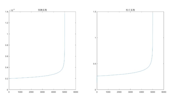
The figures show that when the step count exceeds 4000, the weight function values of both prediction and correction coefficients increase significantly. We can therefore roughly determine that the number of steps to preserve is $5000 - 4000 = 1000$, meaning the preserved integral interval $T$ should be at least 0.2.
We first examine the accuracy of the original predictor-corrector algorithm without short memory, on the domain $(0, 1)$, using the Proposed method’s numerical results as the reference.
Predictor-corrector method vs. other methods at various points:
| $t$ | Proposed method | Predictor-corrector | Absolute error | Relative error% |
|---|---|---|---|---|
| 0.2 | -0.00074434 | -0.00074432 | 0.00000002 | -0.00269 |
| 0.4 | -0.010522 | -0.010521 | 0.00000100 | -0.00950 |
| 0.6 | -0.05108 | -0.05107 | 0.00001000 | -0.01958 |
| 0.8 | -0.16592 | -0.16583 | 0.00009000 | -0.05424 |
| 1.0 | -0.46934 | -0.46864 | 0.00070000 | -0.14915 |
The charts show that the predictor-corrector method without short memory still maintains excellent accuracy compared to other methods. We now introduce the short memory principle into the predictor-corrector method, setting the preserved integral interval length to $T$, and observe the numerical solutions for different values of $T$.
Short memory results: $T = 0.2$ to $T = 1.0$, showing $x(1)$, absolute error, relative error%, and runtime/s
| $T$ | $x(1)$ | Absolute error | Relative error% | Runtime/s |
|---|---|---|---|---|
| 0.2 | -0.29587 | 0.17347 | 36.96 | 11.46 |
| 0.3 | -0.37486 | 0.09448 | 20.13 | 24.04 |
| 0.4 | -0.42228 | 0.04706 | 10.03 | 24.78 |
| 0.5 | -0.44837 | 0.02097 | 4.47 | 27.73 |
| 0.6 | -0.46139 | 0.00795 | 1.69 | 37.51 |
| 0.7 | -0.467 | 0.00234 | 0.50 | 39.22 |
| 0.8 | -0.46891 | 0.00043 | 0.09 | 41.00 |
| 0.9 | -0.46927 | 0.00007 | 0.01 | 43.39 |
| 1.0 (no truncation) | -0.46864 | 0.00070 | 0.15 | 45.21 |
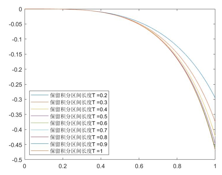
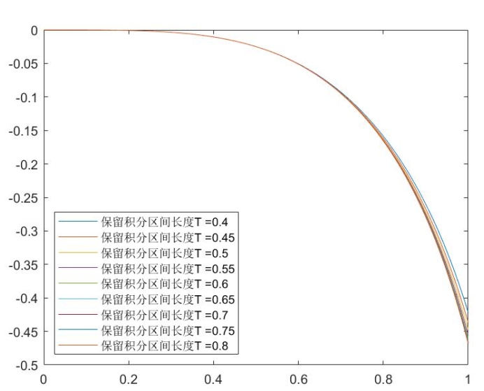
The charts show that for $T < 0.3$, the solution quality is poor, which is consistent with the weight function analysis. When $T = 0.8$, the error is already small enough, so we focus on the range $T = 0.4$ to $0.8$.
Additionally, testing reveals that if only a single step length is preserved for the prediction equation, the resulting accuracy is essentially unaffected. Therefore, we can greatly reduce computation. This is defined as the improved predictor-corrector method.
Improved method results: $T = 0.4$ to $T = 1.0$
| $T$ | $x(1)=$ | Absolute error | Relative error | Runtime/s |
|---|---|---|---|---|
| 0.4 | -0.42169 | 0.04765 | 10.15 | 11.76 |
| 0.45 | -0.43678 | 0.03256 | 6.94 | 13.01 |
| 0.5 | -0.44771 | 0.02163 | 4.61 | 13.07 |
| 0.55 | -0.45543 | 0.01391 | 2.96 | 13.36 |
| 0.6 | -0.4607 | 0.00864 | 1.84 | 14.01 |
| 0.65 | -0.46416 | 0.00518 | 1.10 | 15.03 |
| 0.7 | -0.46632 | 0.00302 | 0.64 | 18.18 |
| 0.75 | -0.46757 | 0.00177 | 0.38 | 19.15 |
| 0.8 | -0.46822 | 0.00112 | 0.24 | 19.16 |
| 1.0 (no truncation) | -0.46864 | 0.00070 | 0.15 | 21.05 |
Optimal $T$ selection: optimal $T$ for given allowable errors
| Allowable relative error/% | Optimal $T$ | Actual relative error/% | Runtime/s | Runtime without truncation/s |
|---|---|---|---|---|
| 10 | 0.4 | 10.15 | 11.76 | 45.21 |
| 5 | 0.5 | 4.61 | 13.07 | 45.21 |
| 2 | 0.6 | 1.84 | 14.01 | 45.21 |
| 1 | 0.65 | 1.10 | 15.03 | 45.21 |
The charts confirm that after introducing and continuously improving the short memory principle, computation time is more than halved while keeping accuracy within the allowable range.
2.4.3 Example 3
$$D_*^\alpha x(t) = \dfrac{2}{\Gamma(3-\alpha)} t^{2-\alpha} - x(t) + t^2 - t$$
Initial conditions: $x(0) = 0,\ x’(0) = -1$
Exact solution: $x(t) = t^2 - t$
Using weight function analysis, we first observe the prediction and correction coefficient images for $\alpha = 1.5$. It is found that both coefficients decrease gradually as the independent variable increases, making it impossible to determine the preserved integral length $T$ from the coefficient images alone. 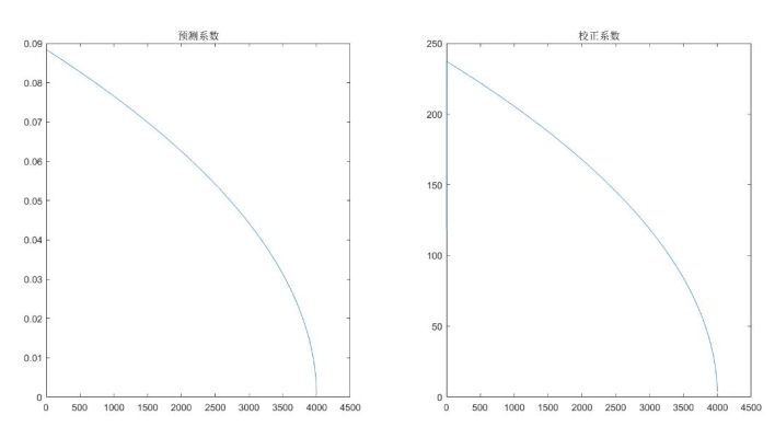
Therefore, we adopt a practical truncation test to determine $T$ step by step. First, we verify the accuracy of the predictor-corrector method without short memory.
$t = 10$ to $t = 50$, exact vs. numerical solutions:
| $t$ | Exact solution | Numerical solution | Absolute error | Relative error% | Runtime/s |
|---|---|---|---|---|---|
| 10 | 90 | 90.1896 | 0.1896 | 0.2107 | 21.3 |
| 20 | 380 | 380.1303 | 0.1303 | 0.0343 | — |
| 30 | 870 | 870.1082 | 0.1082 | 0.0124 | — |
| 40 | 1560 | 1560.0952 | 0.0952 | 0.0061 | — |
| 50 | 2450 | 2450.0865 | 0.0865 | 0.0035 | — |
The predictor-corrector numerical solutions closely approximate the exact solutions, confirming that the predictor-corrector method is applicable to this example.
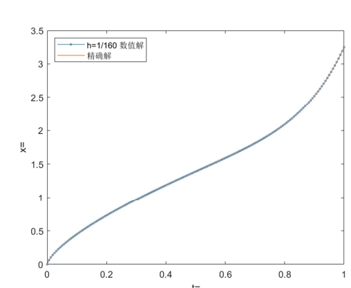
Next, we examine the preserved integral length $T$. At $t = 50$, the exact value is $x(50) = 2450$, with fractional order $\alpha = 1.5$ and step size $h = 1/80$. Let $T$ take values 10, 20, 30, 40, 50 respectively (when $T = 50$, no truncation is applied). The resulting function graphs are:
Short memory method: $T = 10$ to $T = 50$, $x(50)$ and errors
| $T$ | $x(50)$ | Absolute error | Relative error% | Runtime/s |
|---|---|---|---|---|
| 10 | 2411.74 | 38.26 | 1.562 | 3.96 |
| 20 | 2419.30 | 30.70 | 1.253 | 6.91 |
| 30 | 2434.18 | 15.82 | 0.646 | 9.04 |
| 40 | 2434.43 | 15.57 | 0.636 | 10.05 |
| 50 | 2450.09 | 0.09 | 0.004 | 10.83 |
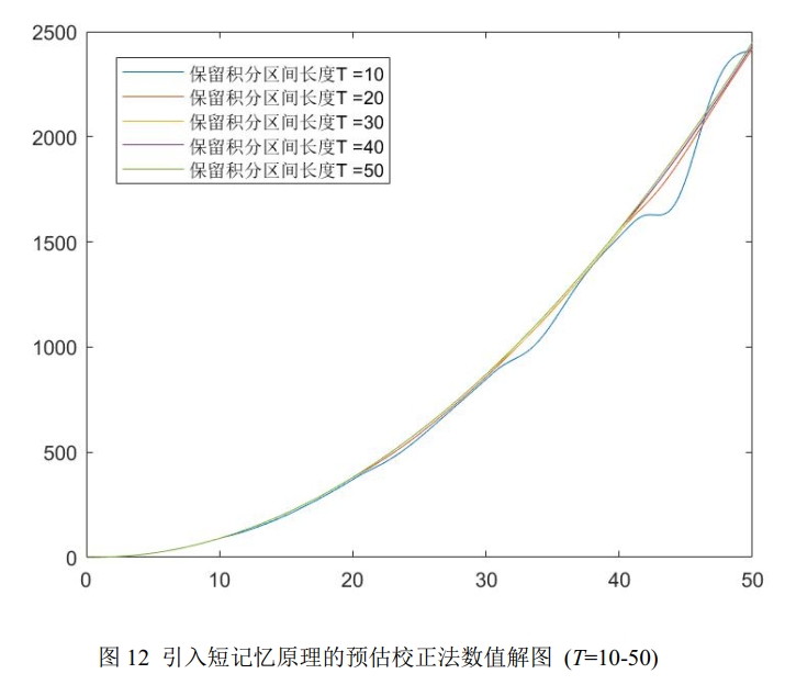
The data shows that when $T = 10$, the function graph still exhibits some oscillation. When $T \ge 20$, the graph stabilizes and the error is sufficiently small. Examining the $T = 10$ case more closely:
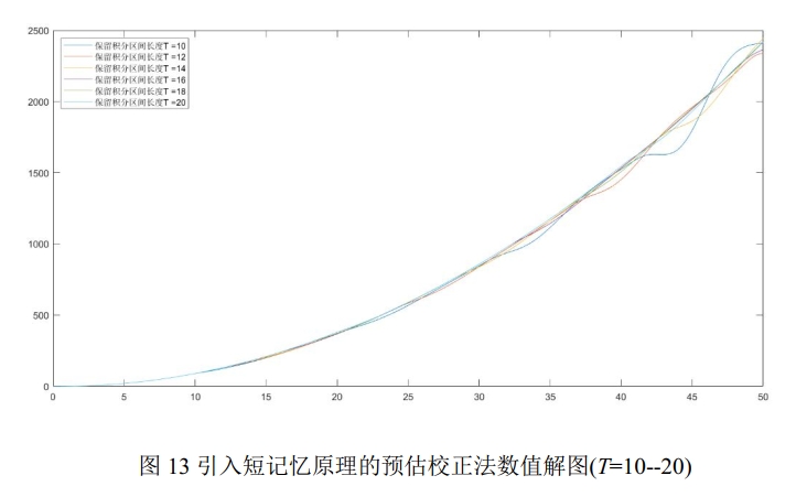
The charts show that oscillation improves after $T = 16$. We now focus on the range $T = 16$ to $20$:
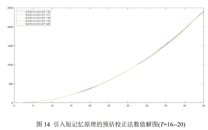
Detailed results for $T = 16$ to $T = 20$
| $T$ | $x(50)$ | Absolute error | Relative error% | Runtime/s |
|---|---|---|---|---|
| 16 | 2364.49 | 85.51 | 3.490 | 5.82 |
| 17 | 2418.09 | 31.91 | 1.302 | 5.85 |
| 18 | 2416.85 | 33.15 | 1.353 | 6.70 |
| 19 | 2415.32 | 34.68 | 1.416 | 9.64 |
| 20 | 2419.30 | 30.70 | 1.253 | 13.69 |
The tables show that $T = 17$ provides acceptable accuracy, so this memory length is adopted.
Comparison: non-truncated long memory $T = 17$ vs. $T = 50$
| $T$ | $x(50)$ | Absolute error | Relative error% | Runtime/s |
|---|---|---|---|---|
| 17 (truncated) | 2418.09 | 31.91 | 1.302 | 3.8 |
| 50 (not truncated) | 2450.0865 | 0.0865 | 0.004 | 21.3 |
This example also shows that at $T = 17$, the short memory principle can significantly reduce computation time.
The predictor-corrector numerical solutions closely approximate the exact solutions. For the short memory method: when $T = 10$, the function graph still shows obvious oscillation; when $T \ge 20$, the graph stabilizes and error is sufficiently small. Examining more closely the range $T = 16$ to $20$, the oscillation clearly improves after $T = 17$. Therefore, subject to function convergence, an integral length $T \ge 17$ can be adopted.
3. Extension to Variable-Order Fractional Systems
3.1 Algorithm
In variable-order fractional differential equations, the constant order $\alpha$ is extended to a time function $\alpha(t)$, i.e.:
$$ D_t^{\alpha(t)} x(t) = f(t, x(t)), \quad x(0) = x_0 $$
At this point, each historical node $t_j$ corresponds to a different order $\alpha(t_j)$, and the weight coefficients must be recalculated at every step. The algorithm is identical to the constant-order case—just replace $\alpha$ with the time-varying function $\alpha(t_j)$ in the loop. When the short memory principle is introduced, we preserve the time-varying weights of the most recent $T$ interval.
3.2 Numerical Examples
3.2.1 Verification of the Predictor-Corrector Method
First, without short memory, we verify whether the predictor-corrector method remains effective for variable-order systems.
Example I ($\alpha(t) = t \cos t$):
$$ D_t^{\alpha(t)} x(t) + x(t) + \sqrt{t} x^2(t) = f(t), \quad x(0) = x’(0) = 0 $$
where $f(t) = t^a \left(1 + t^{\frac{1}{2}+a} + \dfrac{\Gamma(1+a) t^{-\alpha(t)}}{\Gamma(1+a-\alpha(t))} \right), a = 1.2$, and the exact solution is $x(t) = t^a$.
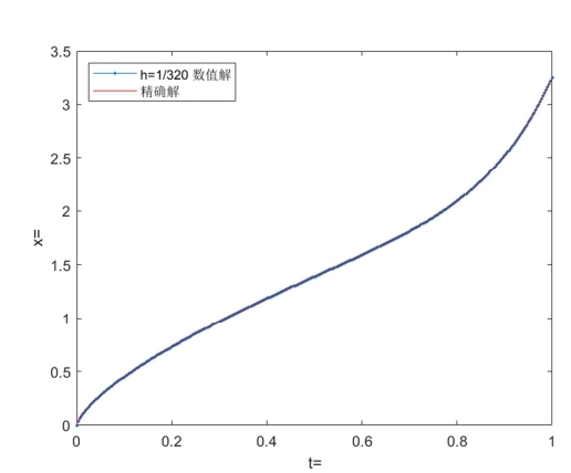
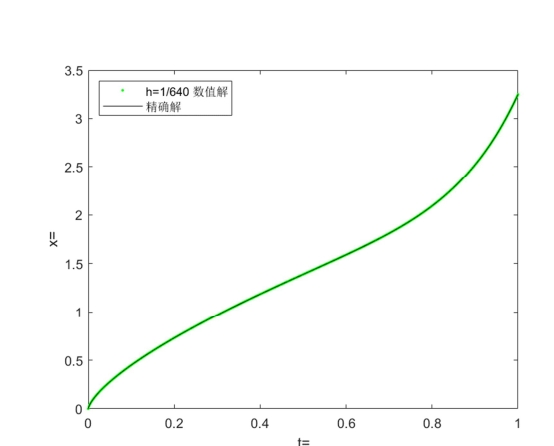
Taking step sizes $h = 1/80,\ 1/160,\ 1/320$, the numerical and exact solutions are compared:
| $t$ | Exact solution | $h=1/80$ numerical | $h=1/80$ rel. error% | $h=1/160$ numerical | $h=1/160$ rel. error% | $h=1/320$ numerical | $h=1/320$ rel. error% |
|---|---|---|---|---|---|---|---|
| 0.1 | 0.0631 | 0.07352 | 16.513 | 0.06644 | 5.293 | 0.06433 | 1.946 |
| 0.2 | 0.1450 | 0.14774 | 1.918 | 0.14585 | 0.614 | 0.14526 | 0.207 |
| 0.4 | 0.3330 | 0.33322 | 0.060 | 0.33300 | -0.006 | 0.33297 | 0.015 |
| 0.6 | 0.5417 | 0.54150 | -0.042 | 0.54157 | -0.030 | 0.54164 | 0.017 |
| 0.8 | 0.7651 | 0.76495 | -0.017 | 0.76498 | -0.013 | 0.76502 | 0.008 |
| 1.0 | 1.0000 | 1.00040 | 0.040 | 1.00010 | 0.010 | 1.00000 | 0.000 |
Smaller step sizes yield higher precision. This confirms that the predictor-corrector method is equally effective for variable-order fractional systems when $\alpha \in (0, 1)$.
Example II ($\alpha(t) = t/2$):
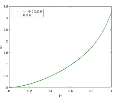
$$ D_t^{\alpha(t)} x(t) = \frac{3 t^{1-\alpha(t)}}{\Gamma(2-\alpha(t))} + \frac{2 t^{2-\alpha(t)}}{\Gamma(3-\alpha(t))}, \quad x(0) = x’(0) = 0 $$
Exact solution: $x(t) = t^2 + 3t$.
| $t$ | Exact solution | $h=1/80$ numerical | $h=1/80$ rel. error% | $h=1/160$ numerical | $h=1/160$ rel. error% | $h=1/320$ numerical | $h=1/320$ rel. error% |
|---|---|---|---|---|---|---|---|
| 0.2 | 0.6400 | 0.63993 | 0.011 | 0.63998 | 0.003 | 0.63999 | 0.002 |
| 0.4 | 1.3600 | 1.35970 | 0.022 | 1.35990 | 0.007 | 1.36000 | 0.000 |
| 0.6 | 2.1600 | 2.15940 | 0.028 | 2.15980 | 0.009 | 2.15990 | 0.005 |
| 0.8 | 3.0400 | 3.03910 | 0.030 | 3.03970 | 0.010 | 3.03990 | 0.003 |
| 1.0 | 4.0000 | 3.99920 | 0.020 | 3.99970 | 0.008 | 3.99990 | 0.003 |
The conclusion is the same as in Example I: reducing step size monotonically improves accuracy.
3.2.2 Verification of the Short Memory Principle
In the constant-order analysis, we already know that when $\alpha < 1$, the prediction and correction weight functions increase nearly linearly in the tail region, and the closer $\alpha$ is to zero, the smaller the early weights. This means the effectiveness of short memory truncation is directly related to $\alpha$. The following variable-order examples verify: the smaller $\alpha$, the shorter the required preserved integral length $T$.
Example I ($\alpha(t) = t \cos t$), taking $h = 1/5000$, progressively truncating the integral interval:
| $T$ | $x(1)$ | Absolute error | Relative error% | Runtime/s |
|---|---|---|---|---|
| 0.2 | 0.7930 | 0.2071 | 20.71 | 9.09 |
| 0.3 | 0.8597 | 0.1403 | 14.03 | 12.37 |
| 0.4 | 0.9006 | 0.0994 | 9.94 | 15.29 |
| 0.5 | 0.9498 | 0.0502 | 5.02 | 17.87 |
| 0.6 | 0.9554 | 0.0446 | 4.46 | 20.30 |
| 0.7 | 0.9673 | 0.0327 | 3.27 | 22.45 |
| 0.8 | 0.9814 | 0.0186 | 1.86 | 23.70 |
| 0.9 | 0.9915 | 0.0085 | 0.85 | 23.89 |
| 1.0 (no truncation) | 1.0051 | 0.0051 | 0.51 | 24.03 |
Testing reveals that preserving only a single step length for the prediction equation has almost no impact on accuracy. The improved results are:
| $T$ | $x(1)$ | Absolute error | Relative error% | Runtime/s |
|---|---|---|---|---|
| 0.2 | 0.7984 | 0.2016 | 20.16 | 4.84 |
| 0.3 | 0.8653 | 0.1347 | 13.47 | 6.65 |
| 0.4 | 0.9064 | 0.0936 | 9.36 | 8.46 |
| 0.5 | 0.9340 | 0.0661 | 6.61 | 9.97 |
| 0.6 | 0.9554 | 0.0446 | 4.46 | 11.36 |
| 0.7 | 0.9732 | 0.0268 | 2.68 | 12.55 |
| 0.8 | 0.9878 | 0.0123 | 1.23 | 13.18 |
| 0.9 | 0.9989 | 0.0011 | 0.11 | 13.29 |
| 1.0 (no truncation) | 1.0053 | 0.0053 | 0.53 | 13.48 |
Within the allowable error range, the improved method maintains high accuracy across $T = 0.4$ to $0.8$.
| Allowable rel. error/% | Optimal $T$ | Actual rel. error/% | Runtime/s | Full-interval runtime/s |
|---|---|---|---|---|
| 10 | 0.4 | 9.36 | 8.46 | 29.38 |
| 5 | 0.6 | 4.46 | 11.36 | 29.38 |
| 2 | 0.8 | 1.23 | 13.18 | 29.38 |
In this example, $\alpha(t) = t \cos t \in [0, 0.5611]$. If we halve the order range to $[0, 0.5101]$ (i.e., $\alpha(t) = \dfrac{t \cos t}{1.1}$), we observe whether the integral length can be further shortened:
| $T$ | $x(1)$ | Absolute error | Relative error% | Runtime/s |
|---|---|---|---|---|
| 0.2 | 0.8301 | 0.1700 | 17.00 | 5.59 |
| 0.3 | 0.8888 | 0.1112 | 11.12 | 13.76 |
| 0.4 | 0.9248 | 0.0752 | 7.52 | 16.15 |
| 0.5 | 0.9490 | 0.0511 | 5.11 | 18.17 |
| 0.6 | 0.9676 | 0.0324 | 3.24 | 22.73 |
| 0.7 | 0.9827 | 0.0173 | 1.73 | 23.31 |
| 0.8 | 0.9946 | 0.0054 | 0.54 | 26.87 |
| 0.9 | 1.0035 | 0.0035 | 0.35 | 27.85 |
| 1.0 (no truncation) | 1.0082 | 0.0082 | 0.82 | 28.11 |
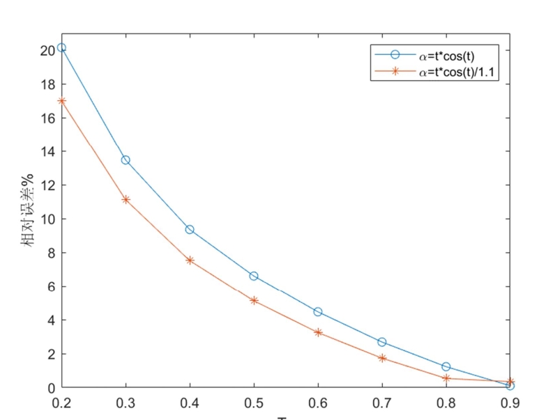
For the same $T$, relative error is noticeably reduced, confirming the conjecture that a smaller $\alpha$ requires a shorter integral length.
Example II ($\alpha(t) = t/2$), taking $h = 1/5000$, exact solution $x(t) = t^2 + 3t$:
| $T$ | $x(1)$ | Absolute error | Relative error% | Runtime/s |
|---|---|---|---|---|
| 0.2 | 2.3370 | 1.6630 | 41.58 | 9.71 |
| 0.3 | 2.7806 | 1.2194 | 30.49 | 24.09 |
| 0.4 | 3.1170 | 0.8830 | 22.08 | 30.12 |
| 0.5 | 3.3802 | 0.6198 | 15.50 | 30.85 |
| 0.6 | 3.5877 | 0.4123 | 10.31 | 35.59 |
| 0.7 | 3.7495 | 0.2505 | 6.26 | 35.72 |
| 0.8 | 3.8722 | 0.1278 | 3.20 | 38.89 |
| 0.9 | 3.9576 | 0.0424 | 1.06 | 38.98 |
| 1.0 (no truncation) | 4.0000 | 0.0000 | 0.00 | 39.82 |
The improved prediction formula yields identical accuracy with significantly reduced computation:
| $T$ | $x(1)$ | Absolute error | Relative error% | Runtime/s |
|---|---|---|---|---|
| 0.2 | 2.3370 | 1.6630 | 41.58 | 4.36 |
| 0.3 | 2.7806 | 1.2194 | 30.49 | 10.00 |
| 0.4 | 3.1170 | 0.8830 | 22.08 | 10.09 |
| 0.5 | 3.3802 | 0.6198 | 15.50 | 10.97 |
| 0.6 | 3.5877 | 0.4123 | 10.31 | 19.20 |
| 0.7 | 3.7495 | 0.2505 | 6.26 | 21.53 |
| 0.8 | 3.8722 | 0.1278 | 3.20 | 23.38 |
| 0.9 | 3.9576 | 0.0424 | 1.06 | 23.48 |
| 1.0 (no truncation) | 4.0000 | 0.0000 | 0.00 | 25.08 |
| Allowable rel. error/% | Optimal $T$ | Actual rel. error/% | Runtime/s | Full-interval runtime/s |
|---|---|---|---|---|
| 10 | 0.6 | 10.31 | 19.20 | 54.06 |
| 5 | 0.8 | 3.20 | 23.38 | 54.06 |
| 2 | 0.9 | 1.06 | 23.48 | 54.06 |
The improved method more than halves computation time, demonstrating the practical value of the short memory principle.
Further reducing the order range from $\alpha \in (0, 0.5)$ to $\alpha \in (0, \frac{1}{3})$ (i.e., $\alpha(t) = t/3$) to verify the same pattern:
| $T$ | $x(1)$ | Absolute error | Relative error% | Runtime/s |
|---|---|---|---|---|
| 0.2 | 2.9046 | 1.0954 | 27.39 | 4.62 |
| 0.3 | 3.2430 | 0.7570 | 18.93 | 10.64 |
| 0.4 | 3.4803 | 0.5197 | 12.99 | 12.86 |
| 0.5 | 3.6539 | 0.3461 | 8.65 | 13.15 |
| 0.6 | 3.7822 | 0.2178 | 5.45 | 15.49 |
| 0.7 | 3.8758 | 0.1242 | 3.11 | 16.52 |
| 0.8 | 3.9416 | 0.0584 | 1.46 | 17.79 |
| 0.9 | 3.9829 | 0.0171 | 0.43 | 19.09 |
| 1.0 (no truncation) | 4.0000 | 0.0000 | 0.00 | 20.51 |
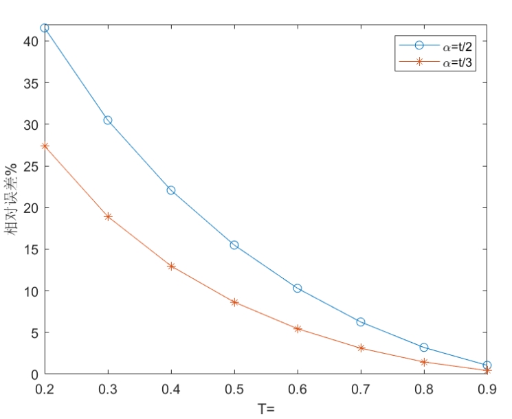
The results again confirm: the smaller $\alpha$, the smaller the relative error at the same $T$, and the better the short memory effect.
4. Key Conclusions and Insights
This thesis combines the short memory principle with the predictor-corrector method to solve variable-order fractional systems. The main conclusions are:
-
The predictor-corrector method is effective for both constant-order and variable-order fractional systems: when $\alpha \in (0, 1)$, the method maintains high accuracy regardless of whether the order is constant or time-varying.
-
Short memory truncation can significantly reduce computation: after introducing the short memory principle, computation time is greatly reduced while maintaining accuracy—the improved predictor-corrector method more than halves the computation time.
-
The qualitative relationship between $\alpha$ and $T$: this is the most important finding of the entire thesis—the smaller $\alpha$, the shorter the integral length $T$ that can be preserved. This means when $\alpha$ is large, only a very short memory interval is needed to achieve the required accuracy, and when $\alpha$ is small, the required memory interval is longer but still far less than the full historical integral. This conclusion provides practical guidance for selecting $T$ under different values of $\alpha$.
-
The short memory strategy is feasible for variable-order systems: by recalculating weight coefficients at each step according to $\alpha(t_j)$, the constant-order predictor-corrector scheme can be extended to variable-order systems, and the short memory strategy remains effective.
These results show that the short memory method is not a universal truncation trick, but a numerical strategy that depends on the fractional order $\alpha$, error tolerance, and problem structure. Its core value lies in providing an analyzable, experimentally verifiable, and extensible framework for variable-order fractional systems.
5. References
[1] Miller, K. S., & Ross, B. (1993). An Introduction to the Fractional Calculus and Fractional Differential Equations. Wiley.
[2] Diethelm, K. (2002). A Predictor-Corrector Approach for the Numerical Solution of Fractional Differential Equations. Nonlinear Dynamics, 29(1-4), 3-22.
[3] Xu, Y., & He, Z. (2011). The short memory principle for solving Abel differential equation of fractional order. Journal of Computational and Applied Mathematics, 5-6.
[4] Parand, K., & Nikarya, M. (2015). New numerical method based on Generalized Bessel function to solve nonlinear Abel fractional differential equation of the first kind. Nonlinear Engineering, 5-7.
[5] Yousefi, F. S., Ordokhani, Y., & Yousefi, S. (2020). Numerical solution of variable order fractional differential equations by using shifted Legendre cardinal functions and Riez method. Engineering with Computers, 6.
[6] Patnaik, S., & Semperlotti, F. (2020). Application of variable and distributed order fractional operators to the dynamic analysis of nonlinear oscillators. Nonlinear Dynamics, 1-2.
[7] Sun, H. G., Chen, W., Wei, H., & Chen, Y. Q. (2011). A comparative study of constant-order and variable-order fractional models in characterizing memory property of systems. The European Physical Journal Special Topics, 2011.
[8] Ma, C. Y., Shiri, B., Wu, G. C., & Baleanu, D. (2018). New fractional signal smoothing equations with short memory and variable order. Signal Processing, 2018.
[9] Wu, F., Gao, R., Liu, J., & Li, C. (2020). New fractional variable-order creep model with short memory. Applied Mathematical Modelling, 2020.