
This article documents the complete problem-solving process for the 2021 Greater Bay Area Financial Mathematics Modeling Competition (Problem B). The core objective is to build an analytical framework that explains stock price fluctuations and assists investment decisions, centered on Bay Area index constituent stocks and incorporating securities research reports, market data, and external environmental information. Around this goal, the paper sequentially designs a Binary Classification Logistic Comprehensive Factor Model, an Event Analysis Model, and a News Sentiment Factor Correction Model, respectively addressing the three problem types: “how to characterize the relationship between factors and future returns,” “how to analyze the impact of external event shocks,” and “how to incorporate sentiment information into a stock selection model.”
1. Problem Restatement
1.1 Background
Securities research reports (sell-side research reports) are analytical documents produced by securities company researchers on the value of securities and related products or factors that influence their market prices. A complete securities research report contains rich information including company operational data, financial projections, valuation results, investment ratings, and risk disclosures, serving as an important reference for investment decision-making.
In recent years, traditional factor models based on financial factors (P/E ratio, market capitalization, etc.) and long-horizon price-volume factors (monthly reversal, monthly trading volume, etc.) have achieved relatively stable excess returns in the A-share market. A factor-based quantitative stock selection model constructed from securities research report feature indicators has become a frontier research topic in the quantitative investment field.
1.2 Problem Description
This research focuses on 10 stocks from the Bay Area index and completes the following four tasks by integrating securities research report information with external market environment data:
- Problem 1: Select securities research reports for 10 Bay Area stocks and extract feature indicators from the reports.
- Problem 2: Model and analyze the impact of securities research report feature indicators on stock trends and propose a clear investment strategy.
- Problem 3: Research the impact of events such as emergencies, public sentiment, and natural disasters on the 10 Bay Area index stocks.
- Problem 4: Integrate securities research reports with external environmental factors, revise the investment strategy from Problem 2, and propose a new investment strategy.
2. Preliminaries: Core Algorithm Principles
This chapter introduces the core algorithms and key terminology that will be directly referenced in subsequent chapters.
2.1 Multi-Class Logistic Regression
Reason for Introduction: In factor-based stock selection, the future movement of a stock is not a simple linear relationship — the three states of price surge, price plunge, and sideways consolidation involve complex non-linear transitions. Traditional linear regression cannot stably characterize such multi-class problems, whereas multi-class logistic regression can provide probability predictions for each class in a multi-class setting and serves as the foundational algorithm for constructing a comprehensive factor.
Basic Model Principle: Multi-class logistic regression performs a linear combination of independent variables and corresponding parameters, then uses a probabilistic model to compute the probability of each class in the dependent variable. Its linear prediction function is:
$$f_k(x) = \beta_{k0} + \beta_{k1}x_1 + \cdots + \beta_{kp}x_p$$
where $\beta_{kj}$ is the regression coefficient, representing the influence of the $j$-th feature on the $k$-th outcome.
After log-odds transformation, the probability of each class is:
$$P(Y=k|X) = \frac{e^{f_k(x)}}{sum_{j=1}^{K} e^{f_j(x)}}$$
Binary Classification Special Case: For $K$ classes, one class is selected as the reference class, and the remaining $K-1$ classes are paired with the reference class to build binary logistic regressions. If class 1 is chosen as the reference, the binary classification of class $l$ ($l \neq 1$) versus class 1 can be expressed as:
$$\ln \frac{P(Y=l|X)}{P(Y=1|X)} = \beta_{l0} + \beta_{l1}x_1 + \cdots + \beta_{lp}x_p$$
Application in This Study: In the factor grouping strategy, stocks are classified into three categories based on future price movements — plunge ($y=-1$), surge ($y=1$), and no extreme movement ($y=0$). Using 24 factor values as explanatory variables, the probability of each category is predicted for every stock. The comprehensive factor value is:
$$F(x) = \frac{1}{1 + \exp(-\beta_1 \cdot x)} - \frac{1}{1 + \exp(\beta_{-1} \cdot x)}$$
2.2 Foundations of Factor Models
Relationship Between Factors and Feature Indicators: In quantitative investment, “factor” and “feature indicator” are essentially two expressions of the same concept. A factor is a variable used to explain differences in stock returns, enabling stocks to be ranked and grouped based on factor values.
Core Idea of Factor Models: Factor models assume that stock returns are driven by several common factors; stocks with similar factor exposures should exhibit similar return performance. By constructing effective factors, expected stock return ranking and grouped trading can be achieved.
Constructing a Comprehensive Factor: A single factor often fails to comprehensively characterize a stock’s return profile, so multiple effective factors need to be weighted and combined to form a comprehensive factor. In this study, the comprehensive factor is derived from 24 securities research report feature indicators compressed through multi-class logistic regression, overlaid with external sentiment factors, forming a comprehensive scoring system.
2.3 Event Study Method
Reason for Introduction: The event study method is an empirical research technique first applied in the financial field. It uses financial market data to quantitatively analyze the impact of specific events on a company’s value. The method is theoretically rigorous, logically clear, and computationally straightforward, making it widely used for studying the impact of external shocks on stock prices.
Basic Model Principle: The event study method compares the actual return of a security during the event window with its expected return “假设事件未发生” (as if the event had not occurred), with the difference being the abnormal return (AR). This来判断事件对股价的影响方向与程度。
Core Steps:
- Event Selection: Identify the event to be studied and its occurrence time point.
- Window Partition: Divide the time interval into an estimation window (120–35 days before the event) and an event window (5 days before to 40 days after the event).
- Normal Return Estimation: Using the market model (CAPM): $R_{it} = \alpha_i + \beta_i R_{mt} + \varepsilon_{it}$
- Abnormal Return Calculation: $AR_{it} = R_{it} - \hat{R}_{it}$
- Cumulative Abnormal Return: $CAR_{cum} = \sum_{t} \bar{A}_t$
- Significance Testing: If the P-value is less than 0.05, the event is considered to have a significant impact on stock price fluctuations.
Application in This Study: Using the 2018 Changsheng Bio-vaccine fraud event as a case study, the 10 stocks are grouped by Shenwan industry classification, and the cumulative abnormal returns of each industry portfolio within the event window are analyzed.
3. Problem Analysis
3.1 Analysis of Problem 1
Problem 1 requires selecting securities research reports for 10 Bay Area stocks and extracting feature indicators from them. Python web scraping is used to collect individual stock research reports from the East Money website over the past three years. Report content is read and feature indicator frequencies are counted, with specific values and definitions obtained from the Shenzhen Tianruan Technology database, serving as an important data source for the Problem 2 analysis.
3.2 Analysis of Problem 2
Problem 2 requires analyzing the impact of research report feature indicators on stock trends and proposing an investment strategy. Due to the non-linear relationship between feature indicators and stock trends, linear regression cannot provide stable predictions. Therefore, machine learning methods are adopted. First, candidate factors are tested for validity using a correlation matrix to assess inter-indicator correlations. Then a multi-class logistic regression model is established to build a regression relationship between factor values and next-period returns, constructing a comprehensive factor verified through grouped testing, ultimately forming a clear investment strategy.
3.3 Analysis of Problem 3
Problem 3 requires building a model to investigate the impact of external factors on the selected 10 stocks. This study proceeds from two angles:
- Macro Analysis Angle: Using the event study method, feature indicators are introduced to analyze the impact of external factors on the 10 stocks.
- Behavioral Finance Angle: From the perspective of behavioral finance theory, news sentiment factors are挖掘 and a factor model is constructed.
The two angles complement each other in jointly explaining the mechanism by which external factors affect individual stocks.
3.4 Analysis of Problem 4
The news sentiment factor from Problem 3 is integrated into the factor model from Problem 2 to reconstruct a comprehensive framework, and the 10 stocks are backtested. By comparing the grouping effects and return performance before and after incorporating the sentiment factor, the superiority of the new model is verified, and an improved investment strategy is proposed.
4. Model Assumptions
- The correlation relationships among research report feature indicators are stable. To avoid using future data, the correlation matrix uses research report data from 2013 (the initial period).
- The relationship between research report data and returns is non-linear. A linear relationship cannot stably predict the relationship between research report data and returns, necessitating the construction of non-linear relationships, for which machine learning provides technical support.
5. Notation
| Symbol | Meaning |
|---|---|
| $R_i$ | Daily return of each sample stock |
| $R_m$ | Market return |
| $AR_i$ | Abnormal return of each sample stock |
| $CAR$ | Portfolio average abnormal return |
| $CAR_{cum}$ | Portfolio cumulative average abnormal return |
6. Model Construction and Solution
6.1 Model for Problem 1 — Construction and Solution
6.1.1 Selection of Research Subjects
This paper selected 10 stocks from the Bay Area index pool as research subjects, covering multiple Shenwan Level-1 industries including electronics, pharmaceuticals, real estate, and building materials:
| Stock Name | Stock Code | Stock Name | Stock Code |
|---|---|---|---|
| EVE Energy | SZ300014 | Huafa Shares | SH600325 |
| Luxshare Precision | SZ002475 | Tower Group | SZ002233 |
| Nationstar Optics | SZ002449 | MiYon | SZ002303 |
| Sunlord Electronics | SZ002138 | Livzon Group | SZ000513 |
| Everwin Precision | SZ300115 | China National | SZ000028 |
6.1.2 Data Acquisition: Python Web Scraping for Research Reports
The core of Problem 1 is to systematically collect research report materials for the 10 stocks. The East Money Data Center’s individual stock research report page is used. The approach involves first locating the research report URL for each stock, then using a Python crawler to scrape historical research report PDFs for each stock over the past three years. A total of 294 research reports are collected, on which subsequent text cleaning, word segmentation, and feature extraction are based. The supplementary files text.xlsx and 解释变量_dwq.xlsx mentioned in the original paper correspond to the research report text organization results and the explanatory variable data used for subsequent factor modeling.
The entire data acquisition process is divided into three steps: Step 1 scrapes research report PDF links, Step 2 extracts PDF text content, and Step 3 performs word segmentation and feature frequency statistics on the research report text. The code function below scrapes research report PDF download links from the East Money research report list page, extracts them using regular expressions, and saves them to an Excel file (links.xlsx).
import urllib
import urllib.request
import re
import pandas as pd

links = []
stocks = ['300014', '002475', '002449', '002138', '300115',
          '600325', '002233', '002303', '000513', '000028']
for i in range(len(stocks)):
    url = "http://data.eastmoney.com/report/" + stocks[i] + ".html"
    data = urllib.request.urlopen(url).read().decode('UTF-8')
    linkre = re.compile(r'\w*AP20\w*')
    list1 = linkre.findall(data)
    for q in list1:
        pdf_url = 'https://pdf.dfcfw.com/pdf/H3_' + q + '_1.pdf'
        links.append(pdf_url)

pd.DataFrame(links).to_excel("links.xlsx")
The following code reads the research report PDF download links, opens each PDF file in sequence, extracts text content using the pdfminer library and concatenates it into a complete string, stores it in a list, and exports it as an Excel file (text.xlsx).
from pdfminer.pdfparser import PDFParser, PDFDocument
from pdfminer.pdfinterp import PDFResourceManager, PDFPageInterpreter
from pdfminer.pdfdevice import PDFDevice
from pdfminer.converter import PDFPageAggregator
from pdfminer.layout import LAParams
import pandas as pd

links_df = pd.read_excel("links.xlsx")
text_list = []
for url in links_df[0]:
    try:
        fp = urllib.request.urlopen(url)
        parser = PDFParser(fp)
        doc = PDFDocument(parser)
        parser.set_document(doc)
        doc.set_parser(parser)
        doc.initialize()
        resource = PDFResourceManager()
        device = PDFPageAggregator(resource, laparams=LAParams())
        interpreter = PDFPageInterpreter(resource, device)
        texts = []
        for page in doc.get_pages():
            interpreter.process_page(page)
            layout = device.get_result()
            for obj in layout:
                if hasattr(obj, 'get_text'):
                    texts.append(obj.get_text())
        text_str = ''.join(texts)
        text_list.append(text_str)
    except:
        text_list.append('')
pd.DataFrame(text_list).to_excel("text.xlsx")
The following code reads research report text content, uses the jieba word segmentation tool to count the occurrences of 35 pre-set feature indicators in each research report, and obtains the feature frequency statistics for each indicator.
import jieba
import pandas as pd
import collections

with open("研报内容.txt", encoding='utf-8') as f:
    data = f.read()
jieba.load_userdict("词典.txt")
seg_list = jieba.lcut(data)
counter = collections.Counter(seg_list)

# Count frequencies of 35 feature indicators
keywords = ['市场', '系统性风险', '市盈率', '市净率', '市销率', 'PEG', '净利润增长率',
             '净资产增长率', '毛利率', '净资产收益率', '销售净利率', '涨跌幅', '换手率', '流通市值', '总市值', '流通股本', '总股本', '盈利预测调整']
result = [counter[k] for k in keywords]
pd.DataFrame(result).to_excel("特征频率.xlsx")
6.1.3 Frequency Statistics of Research Report Feature Indicators
After obtaining all research report texts, the next step is to count the occurrence frequencies of the example indicators in the research reports. The paper categorizes these feature indicators into categories such as overall market, valuation factors, growth factors, profitability factors, momentum reversal factors, trading activity factors, size factors, price volatility factors, and analyst forecast factors, with frequencies individually tallied for each of the 35 example indicators.
From the results, the occurrence frequencies of different indicators in the research reports vary widely. Some indicators are high-frequency words in research reports, such as market factors, gross margin, net sales margin, and total share capital; while some indicators barely appear during the sample period, such as price-to-cash ratio, free-float market cap, forecast net profit growth rate, and earnings expectation adjustments. This frequency distribution itself helps determine which indicators are more worth including in subsequent modeling.
The occurrence frequencies of the 35 example indicators across 294 research reports are as follows:
| Factor Name | Frequency | Factor Name | Frequency |
|---|---|---|---|
| Market Factor | 2391 | Asset Return Rate | 50 |
| Systematic Risk | 5 | Operating Expense Ratio | 0 |
| P/E Ratio | 209 | Financial Expense Ratio | 0 |
| P/B Ratio | 150 | EBIT to Operating Revenue Ratio | 0 |
| P/S Ratio | 27 | Prior Price Change Magnitude | 425 |
| Price-to-Cash Ratio | 0 | Prior Turnover Rate | 70 |
| Enterprise Value Multiple | 0 | Volume Ratio | 0 |
| PEG | 58 | Free-Float Market Cap | 165 |
| Revenue Growth Rate | 128 | Total Market Cap | 322 |
| Operating Profit Growth Rate | 59 | Free-Float Shares | 0 |
| Net Profit Growth Rate | 171 | Total Shares | 389 |
| EPS Growth Rate | 0 | Prior Price Volatility | 0 |
| Net Asset Growth Rate | 44 | Daily Return Std Dev | 0 |
| Shareholders’ Equity Growth Rate | 3 | Forecast Net Profit Growth | 0 |
| Operating Cash Flow Growth Rate | 0 | Forecast Main Business Growth | 0 |
| Net Sales Margin | 671 | Earnings Expectation Adjustment | 0 |
| Gross Margin | 1662 |
6.1.4 Definition and Screening of Feature Indicators
After frequency statistics, the paper does not directly throw all indicators into modeling. Instead, it first conducts further analysis on indicators with “frequency greater than 0.” On one hand, the specific definitions of these indicators are read from the Shenzhen Tianruan Technology database; on the other hand, combined with the common interpretation framework in finance, these indicators are placed back into their respective factor categories for understanding.
From the specific definitions, these indicators can be summarized into the following categories:
Market Factors
- Market Factor: The total share-capital weighted price change of CSI 300 index constituent stocks from the end of month t-1 to the end of month t.
- Systematic Risk: Obtained by regressing the log-return series of individual stocks versus the CSI 300 index from the end of month t-12 to month t; the slope is the systematic risk value.
Valuation Factors
- P/E Ratio: Total market cap at the end of month t divided by net profit over the last 12 months. To control the indicator’s value range, the reciprocal is taken.
- P/B Ratio: The price-to-book ratio at the end of month t (last 12 months, by disclosure date). The reciprocal is taken to control the value range.
- P/S Ratio: The individual stock P/S ratio at the end of month t (last 12 months, by disclosure date). The reciprocal is taken to control the value range.
- PEG: The individual stock PEG at the end of month t (last 12 months).
Growth Factors
- Revenue Growth Rate: Taken from the latest financial report revenue growth rate at the end of month t.
- Operating Profit Growth Rate: Taken from the latest financial report operating profit growth rate at the end of month t.
- Net Profit Growth Rate: Taken from the latest financial report net profit growth rate at the end of month t.
- Net Asset Growth Rate: Taken from the latest financial report net asset growth rate at the end of month t.
- Shareholders’ Equity Growth Rate: Taken from the latest financial report shareholders’ equity growth rate at the end of month t.
Profitability Factors
- Net Sales Margin: Taken from the latest financial report net sales margin at the end of month t.
- Gross Margin: Taken from the latest financial report gross margin at the end of month t.
- Return on Equity (ROE): Taken from the latest financial report return on equity at the end of month t.
- Return on Assets (ROA): Taken from the total assets return rate at the end of month t, calculated as: ROA(%) = [Net Profit + Financial Expenses × (1 − Tax Rate)] / Total Assets × 100.
Trading Factors
- Prior Price Change (1 Month): The price change magnitude from the end of month t to one month prior.
- Prior Price Change (3 Months): The price change magnitude from the end of month t to three months prior.
- Prior Price Change (6 Months): The price change magnitude from the end of month t to six months prior.
- Prior Turnover Rate (1 Month): The frequency of stock turnover in the market during the one month prior to the end of month t.
- Prior Turnover Rate (3 Months): The frequency of stock turnover in the market during the three months prior to the end of month t.
Size Factors
- Free-Float Market Cap: The free-float market cap of the individual stock at the end of month t.
- Total Market Cap: The total market cap of the individual stock at the end of month t.
- Free-Float Shares: The free-float shares of the individual stock at the end of month t.
- Total Shares: The total shares of the individual stock at the end of month t.
After completing the definition review, the specific time-series values of these factors are further read from the Shenzhen Tianruan Technology database. On one hand, this transforms feature indicators from mere “keywords” in research reports into structured variables that can be used for subsequent regression modeling; on the other hand, it provides complete explanatory variable data sources for the factor model in Problem 2.
The final screened valid factors number 24 per the paper’s definition and are used as the core input for the Problem 2 factor model. The counting method here splits prior price change magnitude into 3 indicators (1-month, 3-month, 6-month) and prior turnover rate into 2 indicators (1-month, 3-month).
6.2 Model for Problem 2 — Construction and Solution
6.2.1 Candidate Factors and Data Preprocessing
Before entering Problem 2, the method that will be used repeatedly later is first explained. The multi-class logistic regression method is adopted. It can be understood as an extension of traditional logistic regression, used to predict the probability of a sample falling into different classes.
From here, the paper officially shifts to the “factor construction” perspective. In other words, the research report feature indicators extracted in Problem 1 are uniformly treated as “factors” in this section. The next task is to first check whether these factors are effective, then determine whether there are overly strong correlations among them, and to merge or filter redundant factors.
Monthly-frequency data for 10 stocks from 2013 to 2021 is used. The core model inputs include two parts: (1) next-period (end of month t+1) returns, and (2) current-period (end of month t) 24 factor values. For variables with excessively large values, reciprocal or logarithmic transformations are applied to keep them within a relatively stable numerical range.
6.2.2 Factor Screening and Correlation Testing
When screening factors, a correlation matrix is constructed first. There is one prerequisite assumption: the correlation relationships among the same group of feature indicators are stable over the sample period. To avoid the “look-ahead bias” problem, the correlation matrix uses data from January 2013, i.e., the initial backtesting period.
The correlation coefficient formula is:
$$r(X,Y) = \frac{\mathrm{Cov}(X,Y)}{\sqrt{\mathrm{Var}[X]\mathrm{Var}[Y]}}$$
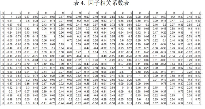
The judgment criterion is straightforward: if the absolute value of the correlation coefficient between any two of the 24 factors exceeds 0.8, it indicates a potentially strong multicollinearity that requires further merging. The final result is that the absolute values of correlation coefficients between all factor pairs are less than 0.8; therefore, all factors are retained and continued into the subsequent machine learning model.
6.2.3 Factor Model Framework Construction
To truly establish the relationship between “current-period factors” and “next-period returns,” the approach from the paper Probability of Price Crashes, Rational Speculative Bubbles, and the Cross Section of Stock Returns is referenced to construct the logistic model.
In the context of Problem 2 modeling, the probabilities of the plunge and surge outcomes can be written as:
$$\Pr_t\left(Y_{i,t,t+12}=-1\right)= \frac{\exp\left(\alpha_{-1}+\beta_{-1}X_{i,t}\right)} {1+\exp\left(\alpha_{-1}+\beta_{-1}X_{i,t}\right)+\exp\left(\alpha_{1}+\beta_{1}X_{i,t}\right)}$$
$$\Pr_t\left(Y_{i,t,t+12}=1\right)= \frac{\exp\left(\alpha_{1}+\beta_{1}X_{i,t}\right)} {1+\exp\left(\alpha_{-1}+\beta_{-1}X_{i,t}\right)+\exp\left(\alpha_{1}+\beta_{1}X_{i,t}\right)}$$
The approach in the referenced paper classifies possible future stock states into three categories: plunge, surge, and non-extreme movements, denoted as -1, 1, and 0 respectively; uses current-period factors as explanatory variables; applies a Logit model to address this multi-class problem; and predicts the future plunge probability. This paper adopts the same approach to construct its own factor Logit model.
Regarding the definition of the dependent variable, very clear rules are also provided: if the decline over the future interval exceeds 50%, it is recorded as a plunge, denoted as -1; if the rise exceeds 100%, it is recorded as a surge, denoted as 1; all other cases are denoted as no extreme movement, 0.
The model training is conducted in a rolling manner. Specifically, at the end of each month t, all monthly-frequency data before t is used to perform one round of multi-class logistic regression. According to the labeling definitions above, plunge and surge are treated as different outcome categories, and regression coefficients are computed accordingly.
The core idea of multi-class logistic regression can be summarized in one sentence: first perform a linear combination of independent variables and parameters, then use a probabilistic model to calculate the probability of a sample falling into different outcome categories. Here, this method is briefly introduced first, then truly applied to the monthly-frequency cross-sectional data of the 10 stocks, with the goal of establishing a non-linear relationship between “current-period factor values” and “next-period return states.”
The code below corresponds to the regression coefficient solving process:
import pandas as pd
import pylab as pl
import numpy as np
from sklearn import datasets
import warnings
import matplotlib.pyplot as plt
from sklearn.linear_model import LinearRegression,LogisticRegression,Ridge,RidgeCV,Lasso, LassoCV
from sklearn.model_selection import train_test_split,GridSearchCV,cross_val_score,cross_validate
from sklearn import metrics as mt
#warnings.filterwarnings('ignore')
# 使文字可以展示
plt.rcParams['font.sans-serif'] = ['SimHei']
# 使负号可以展示
plt.rcParams['axes.unicode_minus'] = False
print('开始')
data_ori = pd.read_excel("解释变量_dwq.xlsx")
data_ori=pd.DataFrame(data_ori)
time = data_ori.iloc[:, -1]
time=time.drop_duplicates()
#print(time)
time1=time.tolist()
#print(time1)
length=len(time1)
#print(length)
list1=[]
n=12
while n < length-12 :
print(n)
t=time1[n]
#print(t)
data=data_ori[(data_ori.时间<=t)]
#print(data)
data_01=data;
data_02=data;
data_01=data_01[(data_01.mark!=-1)]
data_02=data_02[(data_02.mark!=1)]
#print(data)
#print(data_01)
#print(data_02)
data1 = data_01[['mark','市场因子','系统性风险','市盈率','市净率','市销率','PEG',
'"营业利润增长率(%)"','股东权益增长率(%)','销售净利率(%)','销售毛利率(%)','净资产收益率(%)',
'前期涨跌幅1月','前期涨跌幅6月','前期换手率1月','前期换手率3月','流通市值',"'流通股本'"]]
X = data1.iloc[:, 1:]
y = data1.iloc[:, 0]
model = LogisticRegression()
model.fit(X, y.astype('int'))
coef1 = model.coef_ # 回归系数
coef1_icp=model.intercept_
#coef_regression1 = pd.Series(index=['Intercept'] + X.columns.tolist(), data=[model.intercept_[0]] + coef.tolist()[0])
#print(coef1)
a1=coef1[0]
b1=coef1_icp[0]
a1=np.append(a1,b1)
data2 = data_02[['mark','市场因子','系统性风险','市盈率','市净率','市销率','PEG',
'"营业利润增长率(%)"','股东权益增长率(%)','销售净利率(%)','销售毛利率(%)','净资产收益率(%)',
'前期涨跌幅1月','前期涨跌幅6月','前期换手率1月','前期换手率3月','流通市值',"'流通股本'"]]
X2 = data2.iloc[:, 1:]
y2 = data2.iloc[:, 0]
mode2 = LogisticRegression()
mode2.fit(X2, y2.astype('int'))
coef2 = mode2.coef_ # 回归系数
coef2_icp=mode2.intercept_
a2=coef2[0]
b2=coef2_icp[0]
a2=np.append(a2,b2)
a=np.hstack((a1,a2))
an=a.tolist()
an.append(t)
list1.append(an)
#print(an)
n+=1
#for i in tqdm(range(100)):
#sleep(0.01)
#pass
#print(list1)
dt=pd.DataFrame(list1)
dt.to_excel(r'ab.xlsx',sheet_name='测试')
6.2.4 Comprehensive Factor Construction
After obtaining the logistic regression coefficients, the next step is to combine them with the month-t explanatory variable values to construct the comprehensive factor. Here, this comprehensive factor is understood as the plunge probability—that is, an indicator that can rank expected returns.
Let the coefficients from month t-12 be $\alpha_1$, $\alpha_{-1}$, $\beta_1$, $\beta_{-1}$, and the month-t explanatory variables be $X_1$. The formula for the plunge probability is:
$$P_{\text{plunge}}= \frac{\exp\left(\beta_{-1}^{T}X_1+\alpha_{-1}\right)} {\exp\left(\beta_{-1}^{T}X_1+\alpha_{-1}\right)+\exp\left(\beta_{1}^{T}X_1+\alpha_{1}\right)+1}$$
The core meaning of this step is not complicated: through the combination of regression coefficients and current-period factor values, the originally scattered multiple research report features are compressed into a single core indicator that can be directly ranked. The comprehensive factor constructed here essentially corresponds to the plunge probability, or equivalently, an ordered ranking of expected returns, based on which the future return differences of different stocks are compared.
6.2.5 Investment Strategy Design and Backtesting Verification
After obtaining the comprehensive factor, the next step is to first clarify the investment strategy. A monthly portfolio rebalancing approach is adopted: rebalancing is conducted once at the end of each month during 2013–2021, and the 10 stocks are divided into three groups according to the comprehensive factor values. Group 1 has the lowest comprehensive factor values and the highest expected returns; the last group has the highest comprehensive factor values and the lowest expected returns.
At the end of each month t, the specific execution steps are as follows:
- Obtain all dependent variable values (y = 1, -1, or 0) and all explanatory variable values (24 factor values) from before month t.
- Perform multi-class logistic regression on the above data to obtain regression coefficients.
- Calculate the comprehensive factor values.
- Rank each individual stock by comprehensive factor value, and go long on the top 1/3 of stocks with the lowest comprehensive factor to maximize returns.
Where the comprehensive factor calculation formula used in Step 3 is:
$$P_{\text{plunge}}= \frac{\exp\left(\beta_{-1}^{T}X_1+\alpha_{-1}\right)} {\exp\left(\beta_{-1}^{T}X_1+\alpha_{-1}\right)+\exp\left(\beta_{1}^{T}X_1+\alpha_{1}\right)+1}$$
After the strategy is determined, a single-factor backtest is conducted on this approach. The backtest results are as follows:
| Group | Backtest Ending Cumulative Return | Annualized Return | Performance vs. CSI 300 |
|---|---|---|---|
| Group 1 | Above 1517% | 41.6% | Significantly outperforms benchmark |
| Group 2 | Approx. 994% | 34.9% | Significantly outperforms benchmark |
| Group 3 | Approx. 25% | 2.83% | Significantly underperforms benchmark |
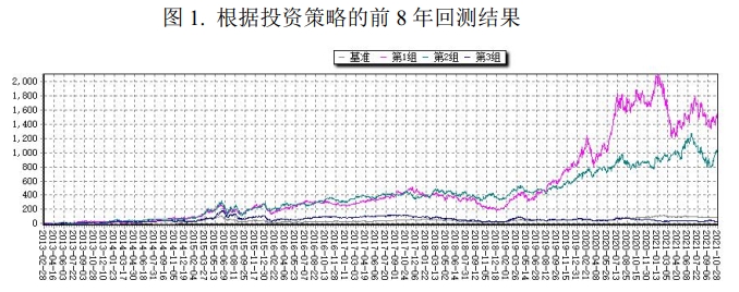
Finally, it can be seen that the constructed comprehensive factor is effective, with significant grouping effects among Groups 1, 2, and 3. This indicates that after ranking by the comprehensive factor and conducting monthly portfolio rebalancing, this investment strategy achieved good return performance on these 10 stocks.
6.3 Model for Problem 3 — Construction and Solution
6.3.1 Mechanism of External Factors’ Impact on Stock Prices
In actual stock market trading, stock movements do not always develop as expected. The reason is that various external shocks continuously emerge in the market, affecting individual stocks and industries to varying degrees. Although many external factors cannot be predicted in advance, we can still summarize patterns by studying market reactions after past events occur, thereby analyzing the relationship between external factors and stock price fluctuations.
In this study, the external factors of interest mainly include emergencies, public sentiment, and natural disasters. From a macro analysis perspective, the event study method can be used to study changes in stock prices after external shocks occur; from a behavioral finance perspective, a news sentiment index can be used to characterize investor attention and sentiment changes, further explaining how external factors affect the stock market.
The logic by which external factors impact stock prices is not complicated. When an emergency occurs, it quickly attracts investor attention and changes market sentiment. Investors make judgments and decisions based on existing information. If a large number of investors react similarly in a short period, stock prices will fluctuate significantly. For this reason, the news sentiment index can reflect both the degree of market attention and the direction of market sentiment, making it an important variable connecting external events and stock price fluctuations.
Based on this thinking, Problem 3 proceeds mainly in two directions: first, building a model based on the event study method to study the impact of specific external events on stock portfolio returns; second, building a model centered on the news sentiment factor to explain the impact of external factors on stock prices from the perspective of sentiment and attention. These two approaches start from different angles but share the same goal: to more systematically understand the relationship between external factors and stock price fluctuations.
6.3.2 Model Construction Based on the Event Study Method
In Problem 3, the first method adopted is the event study method. The event study method was first applied in the financial field. Its core idea is to compare the actual returns of sample stocks during the event window with their “normal returns” as if the event had not occurred, thereby determining whether the event had a significant impact on the stock price.
The event study method’s modeling steps are divided into 12 parts in total, which can be organized into the following key steps:
- Event Selection: Select important events related to industries or individual companies that occurred during the 2013–2021 period.
- Event Date Determination: Determine the time point when the market received the information, and based on this, divide the estimation window and event window. The estimation window is used to estimate normal returns, typically 120 days to 35 days before the event; the event window is flexibly determined based on the possible sustained impact range of the event.
- Research Sample Selection: Select stock samples that may be affected by the event. The research sample in this paper is still the 10 stocks selected earlier, grouped by Shenwan Level-1 industry classification to form industry portfolios, facilitating subsequent comparison of different industries’ reactions to external events.
- Normal Return Estimation: Within the estimation window, the market model is used to calculate the normal returns of stocks. The market model rather than the constant mean adjustment model or market adjustment model is used because the market model provides a more comprehensive explanation and better aligns with common practices in financial research.
- Abnormal Return Calculation: After obtaining normal returns, abnormal returns, portfolio average abnormal returns, and cumulative average abnormal returns within the event window are further calculated to measure the additional impact of event shocks on the stock portfolio.
- Significance Testing: A mean T-test is performed on the cumulative abnormal return series. If the P-value is less than 0.05, it indicates that at the 5% significance level, the event has a significant impact on the sample portfolio’s stock price fluctuations.
This section also requires several key formulas. First, the daily return of an individual stock in the event window can be expressed as:
$$R_{it} = \frac{P_{it} - P_{i,t-1}}{P_{i,t-1}}$$
The market return can be written as:
$$R_{mt} = \frac{I_t - I_{t-1}}{I_{t-1}}$$
In normal return estimation, the market model used is:
$$R_{it} = \alpha_i + \beta_i R_{mt} + \varepsilon_{it}$$
The abnormal return is defined as the difference between the actual return and the normal return:
$$AR_{it} = R_{it} - \hat{R}_{it}$$
The portfolio average abnormal return is:
$$\overline{AR}t = \frac{1}{n}\sum{i=1}^{n} AR_{it}$$
The cumulative average abnormal return is:
$$CAR(t_1,t_2) = \sum_{t=t_1}^{t_2} \overline{AR}_t$$
Through these formulas, the impact of a specific event on an individual stock and industry portfolio can be quantified, and then further tested for significance.
6.3.3 Empirical Design and Model Solution
In the empirical design section, a typical case is selected from common external factors to demonstrate the application process of the event study method. First, the previously selected 10 stocks are classified by Shenwan Level-1 industry. Results show that half of these 10 stocks belong to the electronics industry, 2 belong to the pharmaceuticals and biomedicine industry, and the rest belong to real estate, building materials, and light manufacturing industries.
The corresponding industry classification is shown in the table below:
| Stock Name | Shenwan Level-1 Industry | Stock Name | Shenwan Level-1 Industry |
|---|---|---|---|
| EVE Energy | Shenwan Electronics | Huafa Shares | Shenwan Real Estate |
| Luxshare Precision | Shenwan Electronics | Tower Group | Shenwan Building Materials |
| Nationstar Optics | Shenwan Electronics | MiYon | Shenwan Light Manufacturing |
| Sunlord Electronics | Shenwan Electronics | Livzon Group | Shenwan Pharmaceuticals |
| Everwin Precision | Shenwan Electronics | China National | Shenwan Pharmaceuticals |
Based on this industry structure, the 2018 rabies vaccine fraud incident is重点 selected for the case analysis. The reason for selecting this event is clear: it originated in the pharmaceutical industry but has strong spillover effects, making it more suitable for observing the effectiveness of the event study method in industry shock research.
In specific settings, July 16, 2018 is taken as the event occurrence date; 120 days before the event is set as the estimation window, i.e., February 26, 2018 to July 9, 2018; the event window is set from 5 days before to 40 days after the event. The data source is still the Shenzhen Tianruan Technology database. Since the Bay Area index was established in 2019 and cannot be directly used as the market return benchmark, the CSI 300 index is selected as the market return reference.
In industry grouping, the 10 stocks are further grouped into three categories: electronics and information, pharmaceuticals, and construction. Then, the data for each category of stocks is substituted into the aforementioned event analysis model to calculate the normal return, abnormal return, portfolio average abnormal return, and cumulative average abnormal return of each portfolio within the event window, and based on this, the degree of reaction of different portfolios under the event shock is observed.
After secondary classification according to this definition, the stock portfolio can be organized as follows:
| Stock Name | Industry Category | Stock Name | Industry Category |
|---|---|---|---|
| EVE Energy | Electronics & Info | Huafa Shares | Construction |
| Luxshare Precision | Electronics & Info | Tower Group | Construction |
| Nationstar Optics | Electronics & Info | MiYon | Construction |
| Sunlord Electronics | Electronics & Info | Livzon Group | Pharmaceuticals |
| Everwin Precision | Electronics & Info | China National | Pharmaceuticals |
In the specific case analysis, this part can be further divided into four steps:
- Determine the event occurrence date: Taking the Changsheng Bio vaccine fraud incident reported on July 16, 2018 as the starting point of research.
- Determine the event window: Set 120 days before the event as the estimation window, and from 5 days before to 40 days after the event as the event window.
- Determine the data source: Extract the daily closing prices of individual stocks within the estimation window and event window from the Shenzhen Tianruan Technology database, and use the CSI 300 index as the market return benchmark.
- Substitute into the model for solution: Substitute the data of different portfolio stocks into the event analysis model to calculate normal return, abnormal return, portfolio average abnormal return, and cumulative average abnormal return.
After summarizing the empirical results of the three stock portfolios, they can be organized into the following table:
| Stock Portfolio | T-statistic | P-value | Significance Conclusion | Result Interpretation |
|---|---|---|---|---|
| Pharmaceuticals | 8.085680088 | ≈ 0.00002 | Significant at 95% confidence level | After the emergency, the pharmaceutical portfolio return first declined, then recovered and stabilized as the event was gradually digested. |
| Construction | 11.478369766 | ≈ 0.00003 | Significant at 95% confidence level | The construction portfolio also experienced return reversal and decline after the pharmaceutical event, then gradually rebounded, indicating the sector was also affected by both the event and the broader market. |
| Electronics & Info | -2.062110627 | ≈ 0.045133004 | Significant at 95% confidence level | The electronics portfolio was also impacted by the pharmaceutical industry shock; returns first declined, then went through a period of unstable fluctuations before gradually stabilizing. |
From these three sets of results, it can be seen that emergencies cause significant short-term shocks across different sectors, but the subsequent digestion processes differ. Pharmaceuticals, as the source of the event, experiences the most direct impact; construction and electronics reflect more of a spillover linkage effect. The commonality is that all portfolios experienced return oscillations after the event and eventually gradually moved toward stability.
The significance of this section lies in advancing Problem 3 from “theoretically able to analyze external factors” to “quantitatively verifying the impact of external factors with a specific case.” In other words, the event study method not only provides a research framework but also offers an operational data path for subsequently comparing the degrees of impact across different industry portfolios.
6.3.4 Model Construction and Solution Based on News Sentiment Factors
In addition to the event study method, Problem 3 also introduces news sentiment factors from the perspective of behavioral finance. The core idea here is: if external events significantly affect investor attention and sentiment, then the news headlines themselves can be transformed into a quantifiable explanatory variable to characterize the market’s sentiment changes toward individual stocks.
The construction process of the news sentiment factor is divided into 6 steps:
- Data Acquisition: On a monthly basis, news headlines for the 10 stocks from January 2021 onward are scraped from the East Money website, obtaining a news headline sample set.
- Data Preprocessing: The news headlines in the sample set are segmented using jieba word segmentation, the text is split and connected with spaces; a third-party stop word list is used to process Chinese stop words; then CountVectorizer is used to vectorize Chinese words.
- Construct Training and Test Sets: The sample set is split into training and test sets, and some training set news headlines are manually scored. The scoring rules are:
1for bullish,0for unclear,-1for bearish. - Build Classification Model: Based on the manual scoring, text features are first vectorized, then a Naive Bayes classifier is imported to automatically score the remaining training set news headlines.
- Verify Prediction Accuracy: Data that has not been feature-vectorized is input into the model to check the accuracy of the machine learning predictions.
- Construct Sentiment Factor: The arithmetic mean of the scores of all news headlines for each stock in each month is calculated, obtaining the news sentiment score for that stock in that month, which is defined as the news sentiment indicator—the “sentiment factor” used in subsequent analysis.
Based on this process, a sentiment factor can be constructed for each stock each month. Due to the strong timeliness of sentiment factors, the same logic as in Problem 2 (“using one-year-later plunge/surge results and one-year-earlier factor values for regression”) is no longer directly applicable. Therefore, rather than constructing a completely independent model, the choice is made to修正 Problem 2’s comprehensive factor.
The specific approach is: first calculate the monthly average sentiment factor for the 10 stocks, then test the correlation between $\alpha_1$, $\alpha_{-1}$ in Problem 2 and the sentiment factor, and judge the strength of correlation through $R^2$. The test results are: $R^2$ between $\alpha_1$ and the sentiment factor is 0.4432, and $R^2$ between $\alpha_{-1}$ and the sentiment factor is 0.0859. This indicates a relatively strong relationship between the sentiment factor and $\alpha_1$, while the relationship with $\alpha_{-1}$ is not significant.

Based on this result, the following is substituted:
$$\alpha_1 = -0.0653x - 0.013$$
into the comprehensive factor model from Problem 2. When calculating the comprehensive factor each time, the variable $x$ uses the current-period sentiment factor value of the individual stock, so that the comprehensive factor reflects not only the internal fundamental information of the stock but also the shock brought by external sentiment changes.
From an economic perspective, the role of this correction term is also intuitive: when individual stock sentiment turns from negative to positive, the sentiment factor value $x$ rises, the related term in the model rises, and the individual stock’s plunge probability declines; when individual stock sentiment turns from positive to negative, the sentiment factor value declines, and the individual stock’s plunge probability rises. In other words, the sentiment factor essentially adds a layer of “market sentiment修正” to the comprehensive factor from Problem 2.
Through this processing, the news sentiment factor in Problem 3 is no longer just an auxiliary observation indicator but is truly integrated into the subsequent comprehensive factor modeling framework, laying the foundation for Problem 4’s further integration of internal and external factors.
6.4 Model for Problem 4 — Construction and Solution
6.4.1 Redesign of the Improved Investment Strategy
Based on the new comprehensive factor, the investment strategy in Problem 4 also needs to be restated. At the end of each month t, the rebalancing process can be summarized in the following steps:
Step 1: Obtain all dependent variable values (y = 1, -1, or 0) and all explanatory variable values (24 factor values) from before month t.
Step 2: Perform multi-class logistic regression on the above data to obtain two sets of regression coefficients.
Step 3: Obtain the monthly sentiment factor values, calculate the arithmetic mean of the sentiment factor values for all individual stocks, and then perform OLS fitting between $\alpha$ and the individual stock sentiment factor value $x$, establishing the relationship between $\alpha$ and the individual stock sentiment factor value $x$.
Where the fitted relationship is:
$$\alpha_1 = -0.0653x - 0.013$$
Step 4: Substitute the above equation into the comprehensive factor value to obtain the new comprehensive factor.
Step 5: Rank all individual stocks by comprehensive factor value, and go long on the top 1/3 of stocks with the lowest comprehensive factor to maximize returns.
Compared with Problem 2, the essential change in this strategy is: during monthly rebalancing, not only internal factors are used, but the current-period sentiment factor is also incorporated into the comprehensive factor calculation process, so that the stock selection results simultaneously reflect the company’s internal characteristics and external sentiment changes.
6.4.2 Comparison of Old and New Model Backtest Results and Improvement Analysis
After completing the model modification, the first step is to compare the stock selection effects of the old and new model frameworks using a unified standard. The specific approach is: retain the original grouped backtest framework from Problem 2, still rebalance monthly and group by comprehensive factor ranking, then respectively calculate the return curves and grouping performance of the old comprehensive factor and the new comprehensive factor (with sentiment factor incorporated) within the same time interval. The purpose of this treatment is to make “whether to introduce the sentiment factor” the only variable, so that the changes brought by the model improvement can be more clearly identified.
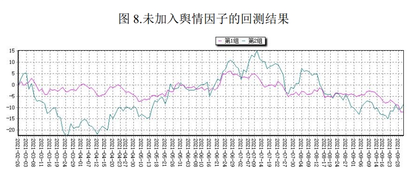
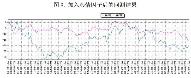
From the backtest results, the new model’s overall performance is better than the old model, mainly reflected in the following aspects:
- Better overall return performance: Against the backdrop of overall market adjustment in 2021, all three groups under the old comprehensive factor grouping experienced significant drawdowns, with Group 1’s drawdown being particularly outstanding; in comparison, the new model’s grouping performance is more stable.
- Clearer group differentiation: During the period from February to September 2021, if the sentiment factor is not introduced, Group 1 and Group 2’s return curves remain entangled for a long time, making it difficult to form an effective differentiation; after incorporating the sentiment factor, Group 1 stocks significantly outperform Group 2 in most of the period.
- Stronger hierarchical stability: Under the new model, the return ranking among different groups is more stable, indicating that the new comprehensive factor can more clearly identify the relative strengths and weaknesses among stocks.
From the analysis of improvement effects, the value of the sentiment factor is mainly concentrated in two points:
- Enhancing factor effectiveness: The sentiment factor strengthens the comprehensive factor’s ability to differentiate stocks’ future performance, making the grouping results more distinguishable.
- Improving adaptability in adverse market environments: When the stock pool declines overall, the new model’s control of Group 1’s drawdown is more effective, indicating stronger adaptability to adverse market environments.
Therefore, the conclusion for Problem 4 can be summarized: after integrating the news sentiment factor into the comprehensive factor model from Problem 2, the new model’s backtest performance is overall better than the old model, and the return performance of Group 1 stocks also improves. This indicates that the new model, when explaining stock price fluctuations, can simultaneously absorb internal fundamental information and external sentiment information, thus possessing stronger practical value.
7. Model Evaluation and Outlook
7.1 Model Strengths
Considering the modeling and empirical results throughout the paper, the main strengths of this factor-based stock selection research are reflected in the following aspects:
- Relatively complete factor integration framework: The model does not rely solely on a single type of information but places research report features, financial and market factors, external events, and news sentiment factors within the same research framework for unified examination, able to simultaneously cover both endogenous and exogenous factors in stock price fluctuations.
- Machine learning methods are suitable for handling complex relationships: Compared with traditional linear methods, multi-class logistic regression can better characterize the non-linear relationship between factor values and future return states, enhancing the model’s ability to capture complex market relationships while retaining statistical interpretability.
- Factor screening process is relatively rigorous: From research report text frequency statistics and Shenzhen Tianruan Technology database factor mapping, to correlation testing and subsequent comprehensive factor construction, the entire process is clearly structured, avoiding redundancy problems caused by simply piling up variables.
- Event study method enhances explanatory power: Beyond factor return prediction, the event study method provides a relatively clear quantitative path for “how external shocks affect stock prices,” enabling the model not only to do return grouping but also to explain the impact of specific events on industries and stock portfolios from a mechanistic perspective.
- Sentiment factor improvement enhances practicality: Problem 4 further introduces news sentiment factors on the basis of the original model, giving the model higher sensitivity when facing market sentiment changes and making the final strategy closer to the real investment environment’s information transmission process.
7.2 Model Limitations
Although the model has demonstrated good grouping effects within the sample, from the perspective of research design and practical application, there are still some limitations that cannot be ignored:
- Relatively small number of sample stocks: The research subjects are mainly 10 Bay Area index constituent stocks. Such a sample size is more suitable for method validation, but the representativeness for a broader market environment is still limited. The model’s generalization ability needs further testing in a larger stock pool.
- Backtest period has阶段性 characteristics: Market style, industry rotation, and external event shocks during the sample period all have strong阶段性 characteristics. Therefore, the current backtest results more illustrate the model’s effectiveness during a specific period and cannot be directly equated with long-term stable effectiveness.
- Sentiment factor has strong timeliness: News headlines and market sentiment changes often spread quickly and decay quickly, meaning sentiment factors may have different effects at different frequencies. If not handled properly, signal lag or noise amplification problems are prone to occur.
- Factor integration method is still relatively linear: Although Problem 4 has incorporated sentiment factors into the comprehensive framework, the current fusion logic still tends to修正 the original comprehensive factor, and the more complex interactive relationships among different types of factors have not been fully explored.
- Real trading constraints have not been fully considered: This paper’s backtest mainly focuses on return performance and grouping effects, with less consideration of real trading conditions such as transaction costs, rebalancing impact, and liquidity constraints. Therefore, when the strategy moves from research conclusions to live trading application, further calibration is needed.
7.3 Improvement Directions
Based on the above limitations, if this research framework is to be further improved in the future, it can be advanced in the following directions:
- Expand external data dimensions: In addition to news sentiment, further introduce external variables such as macroeconomic indicators, industry prosperity, policy events, and fund flows to build a more complete exogenous information characterization system.
- Optimize factor fusion mechanism: Rather than being limited to linear修正 of the original comprehensive factor, attempt to establish a layered fusion or dynamic weighting mechanism, allowing fundamental factors, market factors, and sentiment factors to automatically adjust weights in different market environments.
- Try more diverse machine learning algorithms: While retaining the interpretability of logistic regression, further try ensemble methods such as Random Forest, Gradient Boosting, and XGBoost, and compare the differences in stability, interpretability, and predictive power across different models.
- Expand sample scope for robustness testing: Extend the research subjects from 10 stocks to a larger stock pool, lengthen the backtest time interval, and examine whether the model’s performance remains valid across different market states, sectors, and style environments.
- Add real trading-level verification: In subsequent research, add transaction cost, slippage, turnover rate constraints, and portfolio capacity analysis, further advancing the strategy from “academically effective” to “operationally executable.”
Overall, the factor model constructed in this paper has verified the feasibility of the research approach combining “securities research report feature indicators + external sentiment factors,” and also provided a framework that can be further expanded for the subsequent deeper integration of text mining, event shock analysis, and quantitative stock selection.
8. References
[1] Probability of Price Crashes, Rational Speculative Bubbles, and the Cross Section of Stock Returns. Journal of Financial Economics.
[2] Shenzhen Tianruan Technology Database Technical Documentation.
[3] Shenwan Industry Classification Standard.
Appendix: Core code for each problem is available in the supplementary materials.