
Notes on This Competition Record and Writing
This article is a complete documentation of the solutions for Problem C of the 2020 National College Student Mathematical Contest in Modeling — “Credit Decision Model for Small and Medium Enterprises in the Banking Industry”. In this competition, the author’s responsibilities included: data cleaning and preprocessing, credit strategy development (covering the lending decision model for Problem 1 and the risk evaluation model), and the final report writing and blog-style organization. The decision tree model construction and training was completed by a teammate; this article only introduces the training approach and methodology, without further detailing the procedural steps.
Writing up the problem-solving process as a blog post serves two purposes: first, to systematically organize the modeling ideas for future review and improvement; second, to provide a reference case for students who are equally interested in bank credit risk modeling.
1. Introduction
1.1 Problem Background
For a long time, China’s banking industry has struggled with lending to small and medium enterprises (SMEs), with the core issue being the high credit cost and risk associated with SMEs. Specifically: SMEs are small in scale and lack fixed-asset collateral, making it difficult for banks to directly assess their credit risk. Therefore, banks’ credit decisions for SMEs mainly rely on the enterprises’ transaction票据 (invoice) information and the influence of their upstream and downstream enterprises.
After conducting a reasonable credit risk assessment of SMEs, banks need to formulate a complete credit strategy based on the assessment results, covering dimensions such as whether to grant a loan, loan amount, interest rate, and term. A sound evaluation system is of great significance to banks’ lending decisions.
1.2 Problem Description
This problem provides three attachments: Attachment 1 contains data on 123 enterprises with credit records, Attachment 2 contains data on 302 enterprises without credit records, and Attachment 3 provides 2019 statistical data on the relationship between bank loan annual interest rates and customer churn rates. The task requires completing the following three problems:
- Problem 1: Combine the relevant information of enterprises with credit records to conduct a quantitative analysis of enterprise credit risk, and propose a credit strategy for enterprises under a fixed annual total credit amount.
- Problem 2: Conduct a quantitative analysis of credit risk for enterprises without credit records based on their information, and propose a credit strategy for enterprises under an annual total credit amount of 100 million.
- Problem 3: Comprehensively consider the impact of various sudden factors on enterprises, and propose an optimization plan for the credit strategy in Problem 2.
2. Preliminaries: Core Algorithm Principles
This chapter introduces the algorithm principles that will be directly referenced in subsequent chapters, mainly covering the Analytic Hierarchy Process, fuzzy mathematical evaluation, TOPSIS method, decision tree, and stress testing method.
2.1 Analytic Hierarchy Process (AHP)
1. Reasons for Introducing the Algorithm
When determining the influence weights of each indicator on the decision goal, common issues arise such as the difficulty in quantifying weights and the internal hidden contradictions among weights caused by subjective factors. The Analytic Hierarchy Process (AHP), proposed by American operations researcher Saaty in the 1970s, fundamentally decomposes the related properties of the evaluation object into a target layer, criterion layer, and alternative layer. It performs quantitative and qualitative analysis on fuzzy problems that are difficult to analyze fully quantitatively, to obtain the weight proportion of each layer relative to the highest layer, thereby optimizing the evaluation scheme.
2. 1-9 Scale Method and Judgment Matrix Construction
Indicators are compared pairwise using the 1-9 scale method to construct a judgment matrix $A = (a_{ij})$. Here,
$$a_{ij} = \frac{\text{Importance of the } i \text{ th indicator}}{\text{Importance of the } j \text{ th indicator}}$$
Further written as:
$$A = \begin{pmatrix} a_{11} & a_{12} & \cdots & a_{1n} \ a_{21} & a_{22} & \cdots & a_{2n} \ \vdots & \vdots & \ddots & \vdots \ a_{n1} & a_{n2} & \cdots & a_{nn} \end{pmatrix}$$
3. Weight Computation: Three Methods
Arithmetic mean method:
$$\omega_i = \frac{1}{n} \sum_{j=1}^{n} \frac{a_{ij}}{\sum_{k=1}^{n} a_{kj}}, \quad i = 1,2,\cdots,n$$
Geometric mean method:
$$\omega_i = \frac{\left(\prod_{j=1}^{n} a_{ij}\right)^{1/n}}{\sum_{k=1}^{n} \left(\prod_{j=1}^{n} a_{kj}\right)^{1/n}}, \quad i = 1,2,\cdots,n$$
Eigenvalue method: Find the maximum eigenvalue $\lambda_{\max}$ of the judgment matrix and its corresponding eigenvector, and normalize the eigenvector to obtain the weights.
4. Consistency Check
The consistency index is defined as:
$$CI = \frac{\lambda_{\max}-n}{n-1}$$
The consistency ratio is defined as:
$$CR = \frac{CI}{RI}$$
When $CR < 0.10$, the judgment matrix passes the consistency check; otherwise, the judgment matrix needs to be adjusted.
2.2 Fuzzy Analytic Hierarchy Process (F-AHP)
1. Algorithm Idea
The Fuzzy Analytic Hierarchy Process introduces fuzzy mathematical thinking on the basis of traditional AHP to handle the fuzziness of qualitative indicators. By establishing a fuzzy judgment matrix and fuzzy membership functions, qualitative evaluations are transformed into quantitative scores.
2. Seven-Step Fuzzy Comprehensive Evaluation Model
Taking the supply-demand relationship stability evaluation as an example, the complete process is as follows:
Step 1: Determine the factor set
$$U = {u_1(\text{stable input customer proportion}), u_2(\text{stable output customer proportion}), u_3(\text{variance of average quarterly transaction count})}$$
Step 2: Determine the evaluation set
$$V = {v_1(\text{good}), v_2(\text{fairly good}), v_3(\text{moderate}), v_4(\text{poor})}$$
Step 3: Determine the factor weights
$$A = (a_1, a_2, a_3)$$
Steps 4 to 6: Construct membership functions and form the fuzzy comprehensive judgment matrix
$$R = \begin{pmatrix} r_{11} & r_{12} & r_{13} & r_{14} \ r_{21} & r_{22} & r_{23} & r_{24} \ r_{31} & r_{32} & r_{33} & r_{34} \end{pmatrix}$$
Step 7: Comprehensive evaluation
$$B = A \cdot R = (b_1,b_2,b_3,b_4)$$
2.3 TOPSIS Method
1. Algorithm Principle
TOPSIS (Technique for Order Preference by Similarity to an Ideal Solution) is a multi-attribute decision-making method that ranks alternatives by computing their distances from positive and negative ideal solutions.
2. Complete Calculation Process
Normalization of raw data:
$$z_{ij} = \frac{x_{ij}}{\sqrt{\sum_{i=1}^{n} x_{ij}^2}}, \quad i = 1,2,\cdots,n;\ j = 1,2,\cdots,m$$
Positive and negative ideal solutions:
$$Z^+ = (\max_i z_{i1},\max_i z_{i2},\cdots,\max_i z_{im})$$
$$Z^- = (\min_i z_{i1},\min_i z_{i2},\cdots,\min_i z_{im})$$
Distance computation:
$$D_i^+ = \sqrt{\sum_{j=1}^{m}(Z_j^+ - z_{ij})^2}$$
$$D_i^- = \sqrt{\sum_{j=1}^{m}(Z_j^- - z_{ij})^2}$$
Relative closeness:
$$S_i = \frac{D_i^-}{D_i^+ + D_i^-}, \quad S_i \in [0,1]$$
2.4 Decision Tree
1. Algorithm Overview
A decision tree is a predictive model in the form of an attribute structure, representing a mapping between object attributes and object values. It consists of internal nodes and leaf nodes and is suitable for classification and regression problems.
2. Classification Criteria
Entropy:
$$Entropy(A) = -\sum_{k=1}^{n} p_k \log_2 p_k$$
Information gain:
$$Gain(D,a) = Entropy(D) - \sum_{v=1}^{V} \frac{|D^v|}{|D|} Entropy(D^v)$$
Gini coefficient:
$$Gini(D) = 1 - \sum_{k=1}^{y} p_k^2$$
3. Tree Building Steps
- Treat all samples as a root node.
- Iterate through each candidate variable’s split method and select the optimal split.
- Recursively split nodes until node purity is sufficiently high or stop conditions are met.
4. Model Evaluation Metrics
Accuracy, recall, and F1 score are respectively recorded as:
$$ACC = \frac{TP}{TP + FP}, \quad REC = \frac{TP}{TP + FN}$$
$$PRE = \frac{TP}{TP + FP}, \quad F1 = \frac{2 \times PRE \times REC}{PRE + REC}$$
2.5 Stress Testing Method
1. Methodology
Stress testing is used to evaluate the risk tolerance of financial institutions under extreme unfavorable conditions. In the field of bank credit, it is mainly used to test the impact of sudden factors on enterprise operations.
2. Scenario Testing Process
- Set stress scenarios, such as sudden epidemics, economic recessions, policy changes, etc.
- Identify key impact variables, such as profit growth rate, return rate, etc.
- Simulate the transmission path of impact factors.
- Recalculate risk evaluation values and credit strategies.
3. Problem 1: Credit Strategies for 123 Enterprises with Credit Records
3.1 Enterprise Portrait: Three Core Dimensions
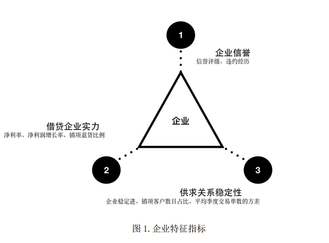
Conduct in-depth analysis of the 123 enterprises with credit records, portraying enterprises from three dimensions:
- Enterprise strength
- Net profit margin: the percentage of net profit to invested capital, comprehensively reflecting business efficiency.
- Net profit growth rate: the magnitude of net profit growth between two time periods, reflecting business performance.
- Output return ratio: the proportion of negative invoice counts to total business counts, reflecting a negative indicator.
- Enterprise credit
- Credit rating: a direct representation of the enterprise’s credit assessment result (A/B/C/D four levels).
- Default history: whether there is a default record, directly affecting enterprise credit.
- Supply-demand relationship stability
- Enterprise stable input customer proportion.
- Enterprise stable output customer proportion.
- Variance of average quarterly transaction count.
3.2 Whether to Lend: Bank Lending Decision Model
3.2.1 Model Structure and Algorithm Flow
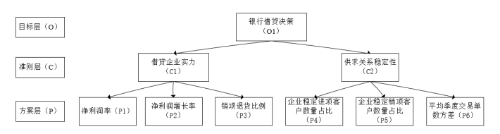
Whether to lend is essentially a multi-attribute comprehensive evaluation problem. For banks, relying solely on a single financial indicator is insufficient to characterize the true creditworthiness of SMEs. Therefore, this article decomposes the enterprise’s lending capacity into two primary dimensions: first, enterprise strength, which reflects business quality, and second, supply-demand relationship stability, which reflects the sustainability of business relationships. The former is mainly composed of net profit margin, net profit growth rate, and output return ratio, while the latter is measured through stable customer proportion and transaction volatility.
Since most indicators in enterprise strength are quantitative, while supply-demand relationship stability contains obvious fuzzy evaluation components, this model does not simply use the fuzzy analytic hierarchy process (F-AHP) alone. Instead, it adopts a comprehensive solution framework of “AHP Weighting + TOPSIS Quantification + F-AHP Fuzzy Comprehensive Evaluation + Time-Weighted Aggregation.” This framework preserves the interpretability of AHP in weight expression while also taking into account the objectivity of TOPSIS in multi-attribute ranking and the F-AHP’s ability to characterize qualitative features.
The hierarchical structure of the model is shown in the figure below:
The overall calculation flow is shown in the figure below:
Input: Enterprise indicator data
  │
  ├─ Step 1: Construct judgment matrices for the target layer, criterion layer, and time layer
  │
  ├─ Step 2: Use AHP to compute primary weights, secondary weights, and time weights, and perform consistency checks
  │
  ├─ Step 3: Use TOPSIS to compute comprehensive scores for the enterprise strength component
  │
  ├─ Step 4: Use F-AHP fuzzy comprehensive evaluation to compute grade scores for the supply-demand relationship stability component
  │
  ├─ Step 5: Weighted synthesis of the two components within the same period to obtain single-period lending capacity evaluation value
  │
  └─ Step 6: Cross-period aggregation using time weights to obtain the final lending evaluation value
Let the three core indicator scores for enterprise strength in time band $i$ be $f_{11}(t_i)$, $f_{12}(t_i)$, and $f_{13}(t_i)$, whose meanings correspond to net profit margin, net profit growth rate, and output return ratio in order. The comprehensive enterprise strength evaluation value can be written as:
$$f_1(t_i) = \omega_{11} f_{11}(t_i) + \omega_{12} f_{12}(t_i) + \omega_{13} f_{13}(t_i)$$
Where $\omega_{11}$, $\omega_{12}$, and $\omega_{13}$ respectively represent the indicator weights of net profit margin, net profit growth rate, and output return ratio within the enterprise strength dimension. The scores of these three underlying indicators are not directly taken from the original values; instead, they are first computed using the TOPSIS analysis method based on the raw indicator values.
For supply-demand relationship stability, denote its comprehensive score in time band $i$ as $f_2(t_i)$. Then the enterprise’s lending capacity evaluation value in that time band is:
$$LEND(t_i) = \omega_{f_1} f_1(t_i) + \omega_{f_2} f_2(t_i)$$
Where $\omega_{f_1}$ and $\omega_{f_2}$ respectively represent the weights of “enterprise strength” and “supply-demand relationship stability” in the criterion layer.
Furthermore, weighted aggregation over the three time bands yields the enterprise’s final comprehensive lending capacity score:
$$LEND = \sum_i \omega_i \cdot LEND(t_i)$$
Where $\omega_i$ is the weight of time band $i$, satisfying $\sum_i \omega_i = 1$. This expression embodies the core idea of this article: the lending capacity of the same enterprise is not a static result at a single point in time, but a weighted synthesis of multiple periods of business performance and supply-demand stability.
3.2.2 Weight Quantification Based on Analytic Hierarchy Process
To make the indicator weights at each layer of the lending decision model clearer, this section elaborates in three layers: “primary criterion layer weights,” “internal weights of enterprise strength,” and “handling of missing indicator scenarios.”
1. Primary Criterion Layer Weights
In the criterion layer, “enterprise strength” and “supply-demand relationship stability” are compared pairwise. Based on business understanding, supply-demand relationship stability better reflects the sustained operational reliability of SMEs, so it is assigned a slightly higher weight than enterprise strength. The corresponding judgment matrix is:
$$A = \begin{pmatrix} 1 & 1/2 \ 2 & 1 \end{pmatrix}$$
When computing weights from the judgment matrix $A$, this article uses all three methods—arithmetic mean, geometric mean, and eigenvalue—for cross-validation:
- Arithmetic mean method:
$$\omega_i^{(1)} = \frac{1}{n} \sum_{j=1}^{n} \frac{a_{ij}}{\sum_{k=1}^{n} a_{kj}}$$
- Geometric mean method:
$$\omega_i^{(2)} = \frac{\left(\prod_{j=1}^{n} a_{ij}\right)^{1/n}}{\sum_{k=1}^{n}\left(\prod_{j=1}^{n} a_{kj}\right)^{1/n}}$$
- Eigenvalue method:
$$A \boldsymbol{\omega}^{(3)} = \lambda_{\max} \boldsymbol{\omega}^{(3)}$$
After finding the dominant eigenvector, normalize it to obtain the corresponding weights.
After synthesizing the three methods, the final weights of the primary criterion layer are:
$$\boldsymbol{\omega} = (\omega_1, \omega_2) = (0.3333, 0.6667)$$
That is, the enterprise strength weight is approximately $1/3$, and the supply-demand relationship stability weight is approximately $2/3$.
For the consistency check, the basic AHP expressions are:
$$CI = \frac{\lambda_{\max} - n}{n - 1}$$
$$CR = \frac{CI}{RI}$$
Since the judgment matrix here is a second-order matrix, when $n=2$, $\lambda_{\max}=2$, thus $CI=0$. Therefore, this matrix naturally satisfies the consistency requirement.
As an implementation reference, the Matlab code for computing weights using the eigenvalue method and completing the consistency check in the analytic hierarchy process is:
%% Analytic Hierarchy Process Consistency Check and Weight Computation
% Input judgment matrix A
[n,n] = size(A);

% Eigenvalue method for weight computation
[V,D] = eig(A);
Max_eig = max(max(D));
[r,c] = find(D == Max_eig, 1);
disp('Eigenvalue method weight results:');
disp(V(:,c) ./ sum(V(:,c)))

% Consistency check
CI = (Max_eig - n) / (n - 1);
RI = [0 0.0001 0.52 0.89 1.12 1.26 1.36 1.41 1.46 1.49 1.52 1.54 1.56 1.58 1.59];
% When n=2, it must be a consistent matrix, so CI = 0.
% To avoid division by zero, replace the second element with a number very close to 0.
CR = CI / RI(n);
disp('Consistency index CI=');
disp(CI);
disp('Consistency ratio CR=');
disp(CR);
if CR < 0.10
    disp('CR<0.10, the consistency of judgment matrix A is acceptable!');
else
    disp('Judgment matrix A needs to be modified!');
end
2. Internal Weights of Enterprise Strength
Within the enterprise strength dimension, the relative weights of net profit margin, net profit growth rate, and output return ratio also need to be further determined. The corresponding judgment matrix is:
$$A_s = \begin{pmatrix} 1 & 1/2 & 3 \ 2 & 1 & 3 \ 1/3 & 1/3 & 1 \end{pmatrix}$$
Its business meaning is: net profit growth rate is slightly higher than net profit margin, both are significantly higher than the output return ratio, but the return ratio still retains some weight because it represents a negative constraint in business quality.
When solving, first normalize the judgment matrix column by column:
$$r_{ij} = \frac{a_{ij}}{\sum_{k=1}^{n} a_{kj}}$$
Then average by row to obtain the approximate weight vector. The final result is:
$$\boldsymbol{\omega}^{(s)} = (0.3108, 0.4934, 0.1958)$$
That is, the weights for net profit margin, net profit growth rate, and output return ratio are 0.3108, 0.4934, and 0.1958 respectively.
Further using the eigenvalue method:
$$\lambda_{\max} = \frac{1}{n} \sum_{i=1}^{n} \frac{(A_s \boldsymbol{\omega}^{(s)})_i}{\omega_i^{(s)}}$$
We obtain:
$$\lambda_{\max} = 3.0536$$
Thus the consistency index is:
$$CI = \frac{3.0536 - 3}{2} = 0.0268, \quad CR = \frac{0.0268}{0.58} = 0.0462 < 0.10$$
This indicates that the judgment matrix has good consistency and is acceptable.
3. Weight Handling in Missing Indicator Scenarios
When some enterprises lack net profit growth rate information, to avoid noise from forced imputation, this article switches to a two-indicator degraded model. The judgment matrix at this point is:
$$A_s’ = \begin{pmatrix} 1 & 3 \ 1/3 & 1 \end{pmatrix}$$
The corresponding weights are:
$$\boldsymbol{\omega}^{(s’)} = (0.75, 0.25)$$
That is, in missing indicator scenarios, the model only uses net profit margin and output return ratio for evaluation, with a higher weight given to net profit margin. This avoids introducing extra noise from missing values while ensuring the model maintains structural consistency and interpretability across different sample conditions.
3.2.3 Time Dimension Weighted Derivation
Enterprise credit is not a static quantity. Compared to earlier years’ data, recent business performance better reflects the enterprise’s current real debt-servicing capacity. Therefore, this article introduces an additional layer of AHP weights in the time dimension, giving higher importance to newer time bands.
The sample time is divided into three time bands:
| Time Band | Corresponding Years |
|---|---|
| $t_1$ | 2016-2017 |
| $t_2$ | 2018 |
| $t_3$ | 2019-2020 |
Under the assumption that “recent information is more important,” the time judgment matrix is constructed as:
$$A_t = \begin{pmatrix} 1 & 1/3 & 1/4 \ 3 & 1 & 1/2 \ 4 & 2 & 1 \end{pmatrix}$$
Following the judgment matrix construction, weight computation, and consistency check steps in the analytic hierarchy process, the time weight vector is:
$$\boldsymbol{\eta} = (\eta_1, \eta_2, \eta_3) = (0.1220, 0.3196, 0.5584)$$
It can be seen that the most recent time band $t_3$ has the highest weight, indicating the model focuses more on the enterprise’s latest business performance.
In the consistency check:
$$\lambda_{\max} = 3.0183, \quad CI = \frac{3.0183 - 3}{2} = 0.00915$$
Taking $RI = 0.52$, then:
$$CR = \frac{0.00915}{0.52} = 0.0176 < 0.10$$
This indicates that the time layer judgment matrix also passes the consistency check.
Therefore, the final lending capacity evaluation value for a single enterprise across the three time bands is:
$$LEND_i = 0.1220 \cdot LEND_i(t_1) + 0.3196 \cdot LEND_i(t_2) + 0.5584 \cdot LEND_i(t_3)$$
This formula clearly embodies the modeling idea that “recent samples are more important.”
3.2.4 Fuzzy Comprehensive Evaluation: Quantification of Supply-Demand Relationship Stability
Supply-demand relationship stability is essentially not a single value, but a concept with fuzzy boundaries. Stable input customer proportion, stable output customer proportion, and variance of average quarterly transaction count all characterize whether the enterprise’s upstream and downstream relationships are stable from different perspectives. However, it is difficult to directly set an absolute “good” or “poor” threshold. Therefore, rather than using simple linear weighting, fuzzy comprehensive evaluation is used here to uniformly map multiple indicators to the same set of evaluation grades.
The factor set for evaluation is taken as:
$$U = {u_1, u_2, u_3} = {\text{stable input customer proportion},\text{stable output customer proportion},\text{variance of average quarterly transaction count}}$$
The evaluation set is taken as:
$$V = {v_1, v_2, v_3, v_4} = {\text{good}, \text{fairly good}, \text{moderate}, \text{poor}}$$
Among them, the first two indicators respectively correspond to the stability of upstream and downstream cooperation relationships, and the third indicator reflects the volatility of transaction rhythm across quarters. The three indicators jointly determine the stability level of the enterprise’s supply-demand relationship.
For weight setting, the results from the analytic hierarchy process are still used. According to the judgment matrix calculation, the weights of the three indicators are:
$$A = (a_1, a_2, a_3) = (0.25, 0.25, 0.5)$$
This means the model places more emphasis on the stability of transaction volatility itself, while giving equal weights to stable input customer proportion and stable output customer proportion.
The corresponding judgment matrix result is:
$$ \begin{pmatrix} 1 & 1 & 2 \ 1 & 1 & 2 \ 1/2 & 1/2 & 1 \end{pmatrix} $$
According to the calculation results in the paper, the maximum eigenvalue of this matrix is $\lambda_{\max}=3$. Further:
$$CI = -4.4409 \times 10^{-16}, \quad CR = -8.5402 \times 10^{-16} < 0.10$$
Therefore, the consistency check passes, and the above weight results are acceptable.
When solving, the membership degrees of each indicator to the four evaluation grades are computed separately. To ensure smooth and interpretable evaluation functions, the conventional assignment method is used, with trapezoidal functions as the membership function model. After obtaining the membership degrees of each single indicator to the evaluation grades, the evaluation results of the three indicators are concatenated to form the enterprise’s fuzzy comprehensive judgment matrix:
$$R = \begin{bmatrix} r_{11} & r_{12} & r_{13} & r_{14} \ r_{21} & r_{22} & r_{23} & r_{24} \ r_{31} & r_{32} & r_{33} & r_{34} \end{bmatrix} = \begin{bmatrix} R_1 \ R_2 \ R_3 \end{bmatrix}$$
Where $r_{ij}$ represents the membership degree of the $i$-th indicator to the $j$-th evaluation grade. Repeating the above steps for each enterprise yields their corresponding fuzzy comprehensive judgment matrices.
Further multiplying the weight vector by the judgment matrix gives the enterprise’s comprehensive membership degree to the four evaluation grades:
$$B = AR = {b_1, b_2, b_3, b_4}$$
If the membership degree corresponding to a certain grade is the largest, the enterprise is classified into that grade. Finally, the four grades are quantified into scores: A, B, C, and D respectively correspond to 100, 80, 60, and 40 points. In this way, the originally difficult-to-directly-measure supply-demand relationship stability is transformed into a quantitative score that can participate in the upper-level lending decision model.
From the model solution results, the fuzzy comprehensive evaluation ultimately generates a supply-demand relationship stability score for each enterprise. According to the example in the paper, the supply-demand stability scores for enterprises No. 1 through No. 10 are: 100, 40, 40, 100, 40, 100, 60, 60, 100, 100. That is to say, the model has already transformed the relatively fuzzy “whether the supply-demand relationship is stable” into a quantitative input that can directly participate in subsequent lending capacity calculations.
As an implementation reference, the following is a Matlab code example for computing the supply-demand relationship stability score using fuzzy comprehensive evaluation:
%% Input: top 10 sales enterprises by year
for i = 1:123
    % 2016-2017 data
    temp = A(find(A(:,1)==i),:);
    temp2017 = temp(find(temp(:,3)<20180000),:);
    temp2017_2 = unique(temp2017(:,2));
    n = histc(temp2017(:,2),temp2017_2);
    n = [temp2017_2,n];
    n = sortrows(n,2);
    n = flipud(n);
    if size(n,1) < 10
        mysort(1:size(n,1),2*i-1:2*i) = n;
    else
        n = n(1:10,1:2);
        mysort(1:10,2*i-1:2*i) = n;
    end
    % 2018 data
    temp2018 = temp(find(temp(:,3)<20190000),:);
    temp2018_2 = unique(temp2018(:,2));
    n = histc(temp2018(:,2),temp2018_2);
    n = [temp2018_2,n];
    n = sortrows(n,2);
    n = flipud(n);
    if size(n,1) < 10
        mysort(11:10+size(n,1),2*i-1:2*i) = n;
    else
        n = n(1:10,1:2);
        mysort(11:20,2*i-1:2*i) = n;
    end
    % 2019 data
    temp2019 = temp(find(temp(:,3)<20200000),:);
    temp2019_2 = unique(temp2019(:,2));
    n = histc(temp2019(:,2),temp2019_2);
    n = [temp2019_2,n];
    n = sortrows(n,2);
    n = flipud(n);
    if size(n,1) < 10
        mysort(21:20+size(n,1),2*i-1:2*i) = n;
    else
        n = n(1:10,1:2);
        mysort(21:30,2*i-1:2*i) = n;
    end
end

%% Output: top 10 sales enterprises by year
for i = 1:123
    % 2016-2017 data
    temp = A2(find(A2(:,1)==i),:);
    temp2017 = temp(find(temp(:,3)<20180000),:);
    temp2017_2 = unique(temp2017(:,2));
    n = histc(temp2017(:,2),temp2017_2);
    n = [temp2017_2,n];
    n = sortrows(n,2);
    n = flipud(n);
    if size(n,1) < 10
        mysort2(1:size(n,1),2*i-1:2*i) = n;
    else
        n = n(1:10,1:2);
        mysort2(1:10,2*i-1:2*i) = n;
    end
    % 2018 data
    temp2018 = temp(find(temp(:,3)<20190000),:);
    temp2018_2 = unique(temp2018(:,2));
    n = histc(temp2018(:,2),temp2018_2);
    n = [temp2018_2,n];
    n = sortrows(n,2);
    n = flipud(n);
    if size(n,1) < 10
        mysort2(11:10+size(n,1),2*i-1:2*i) = n;
    else
        n = n(1:10,1:2);
        mysort2(11:20,2*i-1:2*i) = n;
    end
    % 2019 data
    temp2019 = temp(find(temp(:,3)<20200000),:);
    temp2019_2 = unique(temp2019(:,2));
    n = histc(temp2019(:,2),temp2019_2);
    n = [temp2019_2,n];
    n = sortrows(n,2);
    n = flipud(n);
    if size(n,1) < 10
        mysort2(21:20+size(n,1),2*i-1:2*i) = n;
    else
        n = n(1:10,1:2);
        mysort2(21:30,2*i-1:2*i) = n;
    end
end

%% Compute variance of average monthly transaction count for each enterprise
% Quarterly input counts
mynum1 = [];
for i = 1:123
    temp = A(find(A(:,1)==i),:);
    for j = 1:4
        mynum1(i,j) = size(temp(find(temp(:,3)<20160101+j*300),:),1);
    end
    for j = 1:4
        mynum1(i,4+j) = size(temp(find(temp(:,3)<20170101+j*300),:),1);
    end
    for j = 1:4
        mynum1(i,8+j) = size(temp(find(temp(:,3)<20180101+j*300),:),1);
    end
    for j = 1:4
        mynum1(i,12+j) = size(temp(find(temp(:,3)<20190101+j*300),:),1);
    end
    for j = 1:4
        mynum1(i,16+j) = size(temp(find(temp(:,3)<20200101+j*300),:),1);
    end
end

% Quarterly output counts
mynum2 = [];
for i = 1:123
    temp = A2(find(A2(:,1)==i),:);
    for j = 1:4
        mynum2(i,j) = size(temp(find(temp(:,3)<20160101+j*300),:),1);
    end
    for j = 1:4
        mynum2(i,j+4) = size(temp(find(temp(:,3)<20170101+j*300),:),1);
    end
    for j = 1:4
        mynum2(i,j+8) = size(temp(find(temp(:,3)<20180101+j*300),:),1);
    end
    for j = 1:4
        mynum2(i,j+12) = size(temp(find(temp(:,3)<20190101+j*300),:),1);
    end
    for j = 1:4
        mynum2(i,j+16) = size(temp(find(temp(:,3)<20200101+j*300),:),1);
    end
end

% Total quarterly input and output counts
mynum = mynum1 + mynum2;

% Line charts of quarterly counts for first 20 enterprises
seasontime = 1:20;
for i = 1:20
    subplot(4,5,i)
    plot(seasontime,mynum(i,:),'--o')
    set(gca, 'XTick', 1:1:20)
end

% Compute mean and variance of transaction counts for each enterprise
mymeans = zeros(123,1);
S = zeros(123,1);
for i = 1:123
    temp = mynum(i,:);
    temp(temp==0) = [];   % Remove leading zeros
    mymeans(i) = mean(temp);
    S(i) = sqrt(sum((temp - mean(temp)).^2) / length(temp));
end

%% Compute membership degrees for 123 enterprises to obtain supply-demand relationship stability grades and scores
load percent1.mat
load percent2.mat
percent1 = percent1';
percent2 = percent2';

% Convert benefit-type data to cost-type data
temp_percent1 = 1 - percent1;
temp_percent2 = 1 - percent2;

myA = [0.4 0.4 0.2];   % Weight matrix
scoreindex = zeros(123,2);
for i = 1:123
    R(1,:) = caculate_rate(temp_percent1(:,1),temp_percent1(i,1)); % Obtain indicator P4 membership function value
    R(2,:) = caculate_rate(temp_percent2(:,1),temp_percent2(i,1)); % Obtain indicator P5 membership function value
    R(3,:) = caculate_rate(S,S(i));                                 % Obtain indicator P6 membership function value
    B = myA * R;
    [temp,scoreindex(i)] = max(B);
    % Stability grade score
    if scoreindex(i) == 1
        score2 = 100;
    elseif scoreindex(i) == 2
        score2 = 80;
    elseif scoreindex(i) == 3
        score2 = 60;
    else
        score2 = 40;
    end
    scoreindex(i,2) = score2;
end

%% Append stability scores to enterprise information matrix
company_inf(:,12) = scoreindex(:,2);
3.2.5 TOPSIS Method: Enterprise Strength Quantification Score
Enterprise strength consists of net profit margin, net profit growth rate, and output return ratio, which is a typical multi-attribute comprehensive evaluation problem. To avoid scale bias from direct weighted summation, this article uses TOPSIS for dimensionless processing and ranking.
Let there be $n$ enterprises and $m$ indicators, with the raw data matrix:
$$X = (x_{ij})_{n \times m}$$
First, perform vector normalization:
$$z_{ij} = \frac{x_{ij}}{\sqrt{\sum_{i=1}^{n} x_{ij}^2}}$$
Obtain the normalized matrix $Z = (z_{ij})$.
Then multiply by the indicator weights computed by AHP to form the weighted normalized matrix. Let the weighted normalized matrix be:
For benefit-type indicators (net profit margin, net profit growth rate), larger values are better; for cost-type indicators (output return ratio), smaller values are better. Therefore, the positive ideal solution and negative ideal solution are respectively defined as:
$$Y^+ = (y_1^+, y_2^+, \cdots, y_m^+)$$
$$Y^- = (y_1^-, y_2^-, \cdots, y_m^-)$$
Where benefit-type indicators take the maximum value as the positive ideal solution, and cost-type indicators take the minimum value as the positive ideal solution.
Next, compute the Euclidean distance between each enterprise and the positive and negative ideal solutions:
$$D_i^+ = \sqrt{\sum_{j=1}^{m} (y_{ij} - y_j^+)^2}$$
$$D_i^- = \sqrt{\sum_{j=1}^{m} (y_{ij} - y_j^-)^2}$$
Finally, define the relative closeness:
$$f_1^{(i)}(t) = S_i = \frac{D_i^-}{D_i^+ + D_i^-}$$
Obviously $S_i \in [0,1]$. The larger $S_i$, the closer the enterprise is to the ideal operating state, and the stronger its enterprise strength.
As an implementation reference, the following is a Matlab code example for computing enterprise strength scores using TOPSIS:
%% TOPSIS Score Computation
% Benefit-type indicators are profit margin and profit growth rate
% Cost-type indicator is enterprise return ratio
% Compute the efficacy score for profit margin indicator

% Step 1: Forward normalization of the raw matrix
% Use excel to remove enterprises without data for 2016-17 and import matrix X
load Q1data2016.mat   % X

% 2018
X = company_inf(:,[4:6,10:11]);

% 2019-2020
load Q1data2019-20.mat   % X

%% Start computation
[m,n] = size(X);
disp(['There are ' num2str(m) ' sample data, with ' num2str(n) ' indicators'])
judge = input('Are there indicators that need forward normalization? If yes, enter 1, if no, enter 2: ');
if judge == 1
    position = input('Enter the columns that need forward normalization, e.g., [1,2,3] for columns 1, 2, 3: ');
    type = input('Enter the types of indicators from left to right, 1. cost-type 2. intermediate-type, 3. interval-type, e.g., [2,1,3]: ');
    len = size(type,2);
    for i = 1:len
        if type(i) == 1
            X(:,position(i)) = Min2Max(X(:,position(i)));
            disp(['Column ' num2str(position(i)) ' is a cost-type indicator, forward normalization completed'])
        end
        if type(i) == 2
            best = input(['Enter the best value for column ' num2str(position(i)) ' indicator: ']);
            X(:,position(i)) = Mid2Max(X(:,position(i)),best);
            disp(['Column ' num2str(position(i)) ' is an intermediate-type indicator, forward normalization completed'])
        end
        if type(i) == 3
            best_inter = input(['Enter the best interval for column ' num2str(position(i)) ' indicator (e.g., [10,20]): ']);
            X(:,position(i)) = Inter2Max(X(:,position(i)),best_inter);
            disp(['Column ' num2str(position(i)) ' is an interval-type indicator, forward normalization completed'])
        end
    end
    disp('All indicators have been forward normalized')
end

% Step 2: Normalize the forward matrix
Z = X ./ repmat(sqrt(sum(X.^2)),m,1);

% Step 3: Compute scores and normalize
max_Z = max(Z);
min_Z = min(Z);
judge = input('Do you need to adjust indicator weights? If not, enter 0; if yes, enter 1: ');
if judge == 0
    max_D = sqrt(sum((repmat(max_Z,m,1) - Z).^2,2));
    min_D = sqrt(sum((repmat(min_Z,m,1) - Z).^2,2));
elseif judge == 1
    % w = input('Enter weights from left to right, e.g., [0.3,0.35,0.35]: ');
    % w = [0.25 0.164638129 0.213078843 0.372283029]; % 2016 indicator proportions (no profit growth rate indicator)
    w = [0.103604561 0.164461989 0.146571579 0.213078843 0.372283029];
    max_D = sqrt(sum(repmat(w,m,1) .* (repmat(max_Z,m,1) - Z).^2,2));
    min_D = sqrt(sum(repmat(w,m,1) .* (repmat(min_Z,m,1) - Z).^2,2));
end
score = min_D ./ (max_D + min_D);   % Unnormalized scores
score = score ./ sum(score);        % Normalized scores

%% Compute total scores for all enterprises over three years
fx_score = zeros(123,1);
for i = 1:123
    testsum = sum(temp(:,1)==i) + sum(temp(:,3)==i) + sum(temp(:,5)==i);
    % Enterprise has scores for three years
    if testsum == 3
        myweight = [0.16342 0.29696 0.53961];
        fx_score(i) = myweight * [temp(find(temp(:,1)==i),2); temp(find(temp(:,3)==i),4); temp(find(temp(:,5)==i),6)];
    % Enterprise has scores for two years
    elseif testsum == 2
        % Enterprise has 16-17 scores
        if sum(temp(:,1)==i) == 1
            myweight = [0.3333 0.6667];
            fx_score(i) = myweight * [temp(find(temp(:,1)==i),2); temp(find(temp(:,3)==i),4)];
        % Enterprise has 19-20 scores
        else
            myweight = [0.3333 0.6667];
            fx_score(i) = myweight * [temp(find(temp(:,3)==i),4); temp(find(temp(:,5)==i),6)];
        end
    % Enterprise has only one year of data
    else
        fx_score(i) = temp(find(temp(:,3)==i),4);
    end
end
3.2.6 Comprehensive Evaluation and Grade Threshold Determination
Weighting the enterprise strength score $f_1^{(i)}(t)$ computed by TOPSIS with the supply-demand stability score $f_2^{(i)}(t)$ obtained from fuzzy comprehensive evaluation yields the lending capacity evaluation value for each period. Then, aggregating the results across periods using time weights gives the enterprise’s final comprehensive score $LEND_i$.
For ease of display and subsequent lending decisions, $LEND_i$ is converted to a percentage expression:
$$Score_i = 100 \times LEND_i$$
Then, based on the score distribution and sample ranking results, enterprises are divided into four grades:
| Grade | Comprehensive Score Characteristics | Lending Strategy |
|---|---|---|
| A | High score, stable operations, solid supply-demand relationships | Priority lending |
| B | Relatively high score, controllable risk | Eligible for lending |
| C | Average score, requires prudent evaluation | Lending with reduced quota |
| D | Low score, insufficient debt-servicing capacity and stability | No lending |
If all enterprises are sorted by $LEND_i$ from highest to lowest, the lending threshold can be determined through quantiles or graphical segmentation. In practice, A/B/C grade enterprises can enter the credit pool based on risk appetite, while D grade enterprises are directly excluded.
3.2.7 Solution Results: Whether to Lend
As an implementation reference, the following is a Matlab code example for final bank lending decision scoring:
%% TOPSIS for Credit Decision Model Scoring
% Compute enterprise strength scores
% 2016-2017
load X2.mat
% 2018
load X3.mat
% 2019-2020
load X4.mat

%% Start computation
[m,n] = size(X);
disp(['There are ' num2str(m) ' sample data, with ' num2str(n) ' indicators'])
judge = input('Are there indicators that need forward normalization? If yes, enter 1, if no, enter 2: ');
if judge == 1
    position = input('Enter the columns that need forward normalization, e.g., [1,2,3] for columns 1, 2, 3: ');
    type = input('Enter the types of indicators from left to right, 1. cost-type 2. intermediate-type, 3. interval-type, e.g., [2,1,3]: ');
    len = size(type,2);
    for i = 1:len
        if type(i) == 1
            X(:,position(i)) = Min2Max(X(:,position(i)));
            disp(['Column ' num2str(position(i)) ' is a cost-type indicator, forward normalization completed'])
        end
        if type(i) == 2
            best = input(['Enter the best value for column ' num2str(position(i)) ' indicator: ']);
            X(:,position(i)) = Mid2Max(X(:,position(i)),best);
            disp(['Column ' num2str(position(i)) ' is an intermediate-type indicator, forward normalization completed'])
        end
        if type(i) == 3
            best_inter = input(['Enter the best interval for column ' num2str(position(i)) ' indicator (e.g., [10,20]): ']);
            X(:,position(i)) = Inter2Max(X(:,position(i)),best_inter);
            disp(['Column ' num2str(position(i)) ' is an interval-type indicator, forward normalization completed'])
        end
    end
    disp('All indicators have been forward normalized')
end

% Step 2: Normalize the forward matrix
Z = X ./ repmat(sqrt(sum(X.^2)),m,1);

% Step 3: Compute scores and normalize
max_Z = max(Z);
min_Z = min(Z);
judge = input('Do you need to adjust indicator weights? If not, enter 0; if yes, enter 1: ');
if judge == 0
    max_D = sqrt(sum((repmat(max_Z,m,1) - Z).^2,2));
    min_D = sqrt(sum((repmat(min_Z,m,1) - Z).^2,2));
elseif judge == 1
    % w = input('Enter weights from left to right, e.g., [0.3,0.35,0.35]: ');
    % w = [0.75 0.25]; % 2016 indicator proportions (no profit growth rate indicator)
    w = [0.310813683 0.493385967 0.195800351];
    max_D = sqrt(sum(repmat(w,m,1) .* (repmat(max_Z,m,1) - Z).^2,2));
    min_D = sqrt(sum(repmat(w,m,1) .* (repmat(min_Z,m,1) - Z).^2,2));
end
score = min_D ./ (max_D + min_D);   % Unnormalized scores
score = score ./ sum(score);        % Normalized scores

%% Compute enterprise strength scores for all enterprises over three years
load temp.mat
fx_score = zeros(123,1);
for i = 1:123
    testsum = sum(temp(:,1)==i) + sum(temp(:,3)==i) + sum(temp(:,5)==i);
    % Enterprise has scores for three years
    if testsum == 3
        myweight = [0.16342 0.29696 0.53961];
        fx_score(i) = myweight * [temp(find(temp(:,1)==i),2); temp(find(temp(:,3)==i),4); temp(find(temp(:,5)==i),6)];
    % Enterprise has scores for two years
    elseif testsum == 2
        % Enterprise has 16-17 scores
        if sum(temp(:,1)==i) == 1
            myweight = [0.3333 0.6667];
            fx_score(i) = myweight * [temp(find(temp(:,1)==i),2); temp(find(temp(:,3)==i),4)];
        % Enterprise has 19-20 scores
        else
            myweight = [0.3333 0.6667];
            fx_score(i) = myweight * [temp(find(temp(:,3)==i),4); temp(find(temp(:,5)==i),6)];
        end
    % Enterprise has only one year of data
    else
        fx_score(i) = temp(find(temp(:,3)==i),4);
    end
end
Based on the $LEND_i$ values computed by the model, the 123 enterprises can be classified into four lending grades. The graphical results show that enterprise scores have a relatively clear hierarchical differentiation, indicating that this model can effectively distinguish high-quality enterprises from high-risk enterprises.
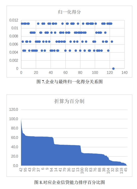
Specifically:
- Grade A enterprises have the strongest lending capacity, with excellent business quality and supply-demand stability, and can be prioritized for loan disbursement.
- Grade B enterprises have overall controllable risk and are suitable as regular credit customers.
- Grade C enterprises, while not obviously high-risk, have shortcomings in business or stability, and lending should be done prudently by reducing quotas and increasing review intensity.
- Grade D enterprises have the lowest scores in comprehensive evaluation, and loan disbursement is not recommended.
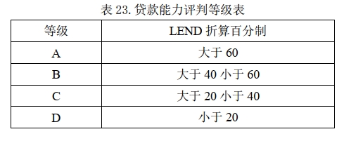
Therefore, the “whether to lend” in Problem 1 can be reduced to a clear classification rule: only grant loans to Grade A, B, and C enterprises, and reject loans for Grade D enterprises. This conclusion provides the prerequisite conditions for subsequent interest rate and quota design.
The following figure shows the final scoring rules formed by this model, which can be used to evaluate other enterprises on the same basis:
3.3 How to Lend: Credit Risk Model for Small and Medium Enterprises
For enterprises that have passed the screening of the lending decision model, the next step is no longer to answer “whether they can get a loan,” but “how they should get a loan.” Therefore, the second model in Problem 1 shifts to risk pricing and quota allocation: on one hand, it continues to preserve enterprise business performance, and on the other hand, it incorporates credit rating and default history into the evaluation system, ultimately forming a risk evaluation value that can be used for interest rate and quota design.
Unlike the lending capacity evaluation value $LEND_i$ in Section 3.2, the enterprise risk evaluation value $RISK_i$ constructed here is for determining loan conditions after passing the initial screening. The two models differ in indicator selection, weight allocation, and result interpretation, so a separate model is needed.
3.3.1 Model Structure and Evaluation Approach
The risk evaluation model still adopts a hierarchical structure of “criterion layer + indicator layer + time layer,” but the criterion layer consists of two parts: “enterprise strength” and “enterprise credit.” Among them, enterprise strength continues to use net profit margin, net profit growth rate, and output return ratio as the three business indicators; enterprise credit is characterized by credit rating and default history. The reason for this approach is: the lending decision model focuses more on whether the enterprise has basic lending eligibility, while the risk evaluation model needs to further answer the question of at what price and quota the bank should bear this risk.
The figure below shows the credit risk model structure established in this article:
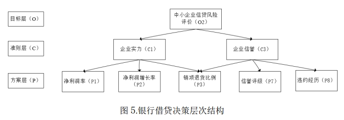
Within a single time band, the risk evaluation value is written as:
$$RISK_i(t) = \omega_1 f_{i1}(t) + \omega_2 f_{i2}(t) + \omega_3 f_{i3}(t) + \omega_4 f_{i4}(t) + \omega_5 f_{i5}(t)$$
Where $f_{i1}(t)$, $f_{i2}(t)$, and $f_{i3}(t)$ respectively represent the scores of net profit margin, net profit growth rate, and output return ratio for enterprise $i$ in time band $t$; $f_{i4}(t)$ and $f_{i5}(t)$ respectively represent the quantitative scores of credit rating and default history; and $\omega_1,\dots,\omega_5$ are the corresponding indicator weights.
Further aggregating over the three time bands yields the enterprise’s final comprehensive risk evaluation value:
$$RISK_i = \eta_1 RISK_i(t_1) + \eta_2 RISK_i(t_2) + \eta_3 RISK_i(t_3)$$
Where $\eta_1, \eta_2, \eta_3$ are the time weights. At this point, the model completes the mapping from single-period business and credit information to the final risk score, and subsequent interest rate and quota design are all based on $RISK_i$.
3.3.2 Weight Quantification Based on Analytic Hierarchy Process
To make the risk evaluation model more interpretable, this article also uses the analytic hierarchy process to quantify weights at each layer, and uses consistency checks to verify the reasonableness of the judgment matrices.
1. Primary Criterion Layer Weights
In the criterion layer, “enterprise strength” and “enterprise credit” are compared pairwise. Compared with pure business performance, credit rating and default history more directly reflect the enterprise’s default risk, so enterprise credit is given higher weight in the risk model. The corresponding judgment matrix can be written as:
$$A_r = \begin{pmatrix} 1 & 1/2 \ 2 & 1 \end{pmatrix}$$
According to the calculation results in the paper, the primary criterion layer weights are:
$$\boldsymbol{\omega}^{(r)} = (0.3333, 0.6667)$$
That is, enterprise strength accounts for 1/3, and enterprise credit accounts for 2/3. Since this judgment matrix is a second-order matrix with a maximum eigenvalue of 2, the consistency naturally satisfies the requirement.
2. Internal Weights of Enterprise Credit
The enterprise credit part is further divided into three indicators: output return ratio, credit rating, and default history. The first retains the negative constraint information in business quality, while the latter two directly characterize the enterprise’s historical credit level. The judgment matrix in the paper is:
$$A_c = \begin{pmatrix} 1 & 1/3 & 1/4 \ 3 & 1 & 1/2 \ 4 & 2 & 1 \end{pmatrix}$$
The computation yields:
$$\lambda_{\max} = 3.0183, \quad CI = 0.00914, \quad CR = 0.01759 < 0.10$$
The consistency check passes, and the corresponding weights are:
$$\boldsymbol{\omega}^{(c)} = (0.1220, 0.3196, 0.5584)$$
This indicates that within the enterprise credit dimension, default history has the strongest explanatory power, followed by credit rating, with output return ratio serving as an auxiliary risk signal in the evaluation.
3. Bottom Indicator Weights of the Risk Model
After combining the primary criterion layer and lower-layer indicator weights, the five bottom indicator weights of the risk evaluation model under normal conditions are obtained:
$$\boldsymbol{\omega} = (0.1036, 0.1645, 0.1466, 0.2131, 0.3722)$$
They correspond in order to net profit margin, net profit growth rate, output return ratio, credit rating, and default history. It can be seen that default history and credit rating have relatively high total weights, which is consistent with the risk model’s goal of “emphasizing credit and historical performance.”
Among them, the enterprise strength part under normal conditions follows the judgment matrix in Section 3.2.2, and its consistency check result is:
$$\lambda_{\max} = 3.0536, \quad CI = 0.0268, \quad CR = 0.0516 < 0.10$$
This indicates that this bottom weight configuration also satisfies the consistency requirement and can be directly used in the risk evaluation model.
When some enterprises lack net profit growth rate, the paper further adopts the degraded model for missing-indicator scenarios. At this point, the four indicator weights are adjusted to:
$$\boldsymbol{\omega}’ = (0.2500, 0.1646, 0.2131, 0.3723)$$
Respectively corresponding to net profit margin, output return ratio, credit rating, and default history. Since this degraded judgment matrix is a second-order matrix with a maximum eigenvalue of 2, consistency naturally holds. This allows the model to maintain structural stability without forced imputation.
3.3.3 Time Dimension Weighting and Risk Score Aggregation
Risk evaluation is also not a static result. The enterprise’s recent business performance and credit status are clearly more valuable as references for the bank’s current pricing than data from earlier years. Therefore, this article continues to use the time judgment matrix from Section 3.2.3 for the time layer, assigning different weights to the three time bands.
The time layer weight vector is:
$$\boldsymbol{\eta} = (\eta_1, \eta_2, \eta_3) = (0.1220, 0.3196, 0.5584)$$
Where the most recent time band $t_3$ has the highest weight, indicating the model places more emphasis on the enterprise’s latest risk status. Therefore, after computing the single-period risk evaluation values for each enterprise across the three time bands, the final comprehensive risk score is:
$$RISK_i = 0.1220 \cdot RISK_i(t_1) + 0.3196 \cdot RISK_i(t_2) + 0.5584 \cdot RISK_i(t_3)$$
From the distribution of the paper’s results, the raw risk evaluation values are relatively concentrated overall. Using them directly for interest rate and quota stratification is not intuitive enough. To enhance the differentiation of scores, the paper further amplifies the raw results and converts them to a percentage scale for subsequent interest rate mapping and grade division. This treatment does not change the relative ranking among enterprises but stretches the scores to a more easily interpretable scale.
3.3.4 Loan Interest Rate Calculation
For interest rate design, the paper adopts the approach of “base rate plus spread pricing.” The base rate references the People’s Bank of China one-year commercial lending rate of 4.35%, and then maps segments within the 4% to 15% range based on enterprise risk scores. The core logic is: the higher the risk score, the better the enterprise quality, so the bank can offer a lower interest rate; the lower the risk score, a higher interest rate is needed to cover the potential risk.
The 13.9866 here comes from the statistical result of the sample risk scores themselves. The specific approach is: first amplify the raw risk evaluation values, then normalize and convert them to a percentage scale to obtain a set of optimized scores more suitable for pricing; then take the average of these percentage scores for the 123 enterprises to obtain 13.9866.
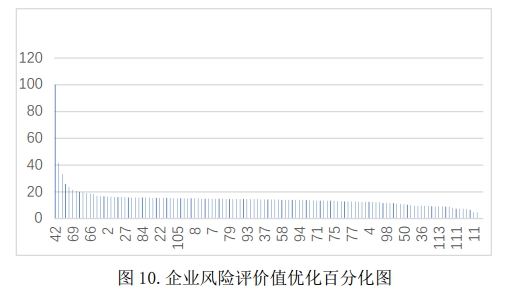
I use this average as the anchor point for the segmented base rate 4.35%. The advantage of this approach is that the segmentation point is not subjectively specified by humans but naturally derived from the overall sample score level. Therefore, the score intervals [0,13.9866) and [13.9866,100] respectively correspond to the two interest rate segments 15%→4.35% and 4.35%→4%. Letting the risk score be $x$ and the loan interest rate be $y$, the interest rate function is written as:
When $x \ge 13.9866$,
$$y = 4.35 - \frac{4.35 - 4}{100 - 13.9866}(x - 13.9866)$$
When $x < 13.9866$,
$$y = 15 - \frac{15 - 4.35}{13.9866}x$$
This mapping approach has two advantages. First, it ensures that the interest rate for high-score enterprises gradually converges toward the low interest rate end, enhancing the sense of gain for high-quality enterprises. Second, it retains sufficient risk premium for low-score enterprises, achieving a balance between revenue and customer churn.
3.3.5 Loan Quota Allocation
For quota design, the paper assumes that the annual total disbursable loan amount is fixed at 100 million, and the per-enterprise loan quota is预设 five tiers: 1 million, 700,000, 500,000, 200,000, and 100,000. To balance risk control and capital utilization efficiency under the total amount constraint, the model does not rigidly segment based on absolute scores but divides quota tiers based on the enterprise’s ranking proportion in the overall population.
The initial quota tiers are:
| Tier | Loan Quota |
|---|---|
| I | 1 million |
| II | 700,000 |
| III | 500,000 |
| IV | 200,000 |
| V | 100,000 |
When allocating quota, I first divide the annual total disbursable amount 100 million into 5 portions, each 20 million, respectively corresponding to the five quota tiers. Then, combined with the enterprise’s risk evaluation value ranking proportion in the overall population, the interval areas corresponding to tiers I, II, III, IV, and V are made consistent, thereby establishing a mapping from “risk evaluation value ranking proportion” to “credit quota tier.”
The mapping relationship is shown in the figure:
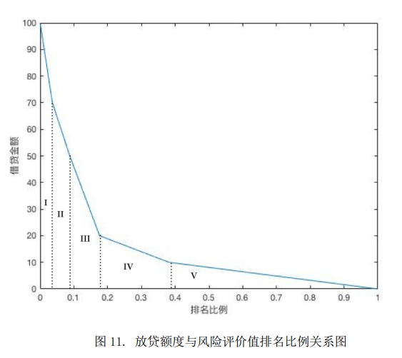
By reversing this path, the ranking proportion intervals corresponding to each quota tier can be obtained, and the final stratification rules are:
| Tier | Loan Quota | Ranking Proportion |
|---|---|---|
| I | 1 million | Top 3.6347% |
| II | 700,000 | Top 8.7844% |
| III | 500,000 | Top 17.6110% |
| IV | 200,000 | Top 38.2090% |
| V | 100,000 | Remaining approved enterprises |
In this way, enterprises with higher risk evaluation values and higher rankings can obtain higher credit quotas; enterprises with relatively lower rankings are allocated more conservative quota levels. This completes the closed loop of the two-stage framework in Problem 1: $LEND_i$ is used to decide whether to lend, and $RISK_i$ is used to decide how to lend.
4. Problem 2: Credit Strategies for 302 Enterprises Without Credit Records
Note: The author was only responsible for data cleaning and credit strategy development. The decision tree model construction and training was completed by a teammate, and this section only introduces the training approach and methodology without further detailing the procedural steps.
4.1 Challenges of Data Missing
Attachment 2’s 302 enterprises do not provide the two key pieces of information — “credit rating” and “default history” — so they cannot be directly substituted into the lending decision model and risk evaluation model already established in Problem 1. That is to say, the core of Problem 2 is not to design a new credit system but to first fill in the missing credit labels, and then put these enterprises back into the two-stage model of Problem 1 for evaluation.
Therefore, the solution approach for this problem can be summarized as two steps: first, use the data of the 123 enterprises with credit records in Attachment 1 to train a classification model and predict the credit ratings and default histories of the enterprises in Attachment 2; second, after supplementing the predictions into the Attachment 2 samples, continue using the integrated “whether to lend + how to lend” framework to complete loan approval, interest rate design, and quota allocation.
4.2 Decision Tree to Fill the Data Gap
4.2.1 Data Preprocessing
During data cleaning, I first use pandas.read_excel() to read all tables in Attachments 1 and 2 and convert them to DataFrame structures. Then, I remove invalidated invoice samples from the “input invoice information” and “output invoice information” to avoid interference from invalid documents on the characterization of enterprise transaction scale and business characteristics.
Next, I sum the “total price and tax” in the four invoice detail tables by “enterprise code” to obtain the total input price-tax amount and total output price-tax amount for each enterprise. Then, these two summary results are added back to the enterprise master table, enabling the original enterprise information table to simultaneously contain business labels and transaction summary characteristics.
Since “credit rating” and “default history” in Attachment 1 are string-type variables, they need to be numerically encoded before entering the model. Here, LabelEncoder is used to re-encode the category labels, and train_test_split is used to divide samples into training, validation, and test sets with a ratio of 3:1:1. Finally, “input price-tax amount” and “output price-tax amount” are used as features to train classification models for predicting “credit rating” and “default history” respectively.
As an implementation reference, the Python code for data cleaning and training set construction is:
import numpy as np
import pandas as pd
from sklearn.preprocessing import LabelEncoder, OneHotEncoder
from sklearn.model_selection import train_test_split
from sklearn.metrics import accuracy_score, recall_score, f1_score
from sklearn.tree import DecisionTreeClassifier, export_graphviz
from sklearn.externals.six import StringIO
import pydotplus
import matplotlib.dates as mdate
from tqdm import tqdm
import matplotlib.pyplot as plt
import os
# Add to environment variable
os.environ['PATH'] += os.pathsep + ''# Environment variable path

# Read and clean the raw data
df_0 = pd.read_excel('Attachment 1: Data on 123 Enterprises with Credit Records.xlsx', sheet_name='Enterprise Information', encoding='gbk')
df_in = pd.read_excel('Attachment 1: Data on 123 Enterprises with Credit Records.xlsx', sheet_name='Input Invoice Information', encoding='gbk')
df_out = pd.read_excel('Attachment 1: Data on 123 Enterprises with Credit Records.xlsx', sheet_name='Output Invoice Information', encoding='gbk')
df_in = df_in[df_in.loc[:, 'Invoice Status'] == 'Valid Invoice']
df_out = df_out[df_out.loc[:, 'Invoice Status'] == 'Valid Invoice']

# Group and sum
sum_in = df_in['Total Price and Tax'].groupby(df_in['Enterprise Code']).sum()
sum_out = df_out['Total Price and Tax'].groupby(df_out['Enterprise Code']).sum()

# Join tables
sum_in = sum_in.to_frame()
sum_out = sum_out.to_frame()
sum_in.rename(columns={'Total Price and Tax': 'Input Price-Tax Total'}, inplace=True)
sum = sum_in.join(sum_out)
df_0.set_index('Enterprise Code', drop=True, inplace=True)
df = df_0.join(sum)

# Encoding
df['Credit Rating'] = LabelEncoder().fit_transform(df['Credit Rating'].values.reshape(-1, 1)).reshape(1, -1)[0]
df['Default History'] = LabelEncoder().fit_transform(df['Default History'].values.reshape(1, -1)[0])
#df.to_csv('123 enterprises.csv')

# Machine learning
from sklearn.model_selection import train_test_split
features = df.drop(['Enterprise Name', 'Credit Rating'], axis=1)
label = df['Default History']
f_v = features.values
f_names = features.columns.values
l_v = label.values
X_tt, X_validation, Y_tt, Y_validation = train_test_split(f_v, l_v, test_size=0.2) # Validation set
X_train, X_test, Y_train, Y_test = train_test_split(X_tt, Y_tt, test_size=0.25) # Test set Due to one splitting, the ratio is adjusted

models = []

#models.append(('LogisticRegression', LogisticRegression(C = 1000, tol = 1e-10, solver = 'sag', max_iter = 10000)))
models.append(('DecisionTreeGini', DecisionTreeClassifier()))
#models.append(('DecisionTreeEntropy', DecisionTreeClassifier(criterion='entropy')))
for (clf_name, clf) in models:
 clf.fit(X_train, Y_train)
 xy_lst = [(X_train, Y_train), (X_validation, Y_validation), (X_test, Y_test)]
 for i in range(len(xy_lst)):
  X_part = xy_lst[i][0]
  Y_part = xy_lst[i][1]
  Y_pred = clf.predict(X_part)
  print(i)
  print(clf_name, 'ACC', accuracy_score(Y_part, Y_pred))
  print(clf_name, 'REC', recall_score(Y_part, Y_pred))
  print(clf_name, 'F1', f1_score(Y_part, Y_pred))
4.2.2 Model Training
The decision tree is chosen as the core machine learning model for this problem for two main reasons: on one hand, the sample size is limited, and decision trees are easier to train on small-sample classification problems; on the other hand, decision trees have strong interpretability, making it easy to directly transform “how purchase and sales scale affect credit rating and default history” into visualized classification rules.
From a principles perspective, decision trees continuously select the optimal feature to split the sample set so that the node purity after each split is as high as possible. Here, classification trees based on the Gini coefficient standard are used to train “credit rating” and “default history” separately.
In the model evaluation stage, accuracy ACC, recall REC, and F1-score are used as the main evaluation metrics, respectively measuring the model’s overall classification accuracy, its ability to identify the target class, and the balance between precision and recall. By training “credit rating” and “default history” separately, the decision tree models for predicting the credit labels of Attachment 2 enterprises can be obtained.
From the implementation results, this code outputs ACC, REC, and F1 metrics on the training, validation, and test sets respectively, where 0, 1, and 2 respectively correspond to training, validation, and test sets. The purpose of doing so is to simultaneously observe the model’s performance on training samples and unseen samples, avoiding the situation of only looking at training results while ignoring generalization ability. Additionally, the model can be further exported as a decision tree diagram to visually display the classification rules.
4.2.3 Prediction Results
After model training is complete, inputting the 302 enterprises from Attachment 2 into the decision tree yields their corresponding “credit rating” and “default history” predicted values. In this way, the originally missing credit labels are filled, and Attachment 2 enterprises have the same field structure as Attachment 1 enterprises, allowing them to continue participating in the subsequent quantitative credit analysis.
From the results, the input price-tax total and output price-tax total have a certain ability to differentiate credit ratings and default histories, providing an approximate credit label for enterprises without historical credit records. Although these prediction results cannot completely replace real historical credit performance, under the limited information provided by the problem, they are sufficient to support subsequent lending decisions and risk pricing.
Further, after filling in the labels, Attachment 2 samples can continue just like in Problem 1 to compute the enterprise strength total score, lending capacity normalized total score, and the annual risk evaluation total scores across the three time bands, ultimately aggregating into a comprehensive risk evaluation value. In this way, the decision tree’s output is no longer just a single classification label but directly becomes an input variable in the subsequent $LEND_i$ and $RISK_i$ calculation chain.
4.3 Credit Strategy Development
After filling in credit ratings and default histories, the 302 enterprises in Attachment 2 can be put back into the credit framework already established in Problem 1 for continued calculation. The specific solution still follows the two main lines of “whether to lend” and “how to lend,” except that the input samples have switched from Attachment 1’s historical credit enterprises to Attachment 2’s enterprises with supplemented labels via decision tree.
1. Whether to Lend
First, compute the lending capacity evaluation value $LEND_i$ using enterprise strength scores and supply-demand relationship stability scores, and normalize and convert to a percentage scale. This yields the lending capacity distribution of the 302 enterprises under the same evaluation standards. Then, based on the grade division standards already determined in Problem 1, determine whether the enterprises are approved for lending. That is to say, the “whether to lend” part of Problem 2 is essentially still judging which of grades A, B, C, and D these enterprises fall into.
The corresponding “whether to lend” visualization results are as follows:
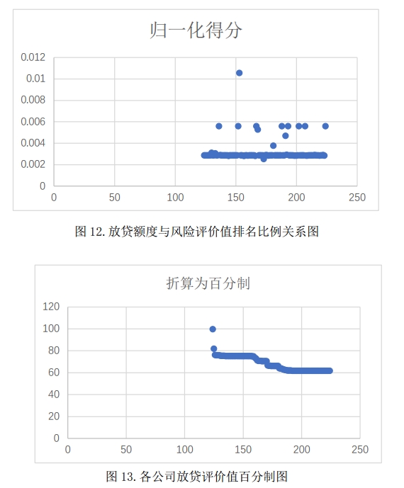
2. Loan Interest Rate
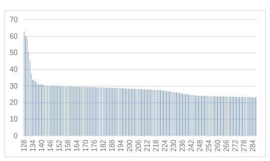
For approved enterprises, continue to compute the comprehensive risk evaluation value, and follow the interest rate allocation approach of Problem 1 for pricing. Here, the method of “anchoring the base rate with the percentage average” is still used, except that the Attachment 2 sample’s percentage score average becomes 23.1107. Therefore, in Problem 2, the interest rate segmentation point is no longer 13.9866 from Problem 1 but is changed to 23.1107 as the anchor for the 4.35% base rate. Enterprises above this average are mapped to the low interest rate interval, while those below the average are mapped to the high interest rate interval.
The corresponding interest rate calculation formula is:
When $x \ge 23.1107$,
$$y = 4.35 - \frac{4.35 - 4}{100 - 23.1107}(x - 23.1107)$$
When $x < 23.1107$,
$$y = 15 - \frac{15 - 4.35}{23.1107}x$$
The corresponding interest rate normalization results are as follows:
3. Loan Quota
For quota allocation, the ranking proportions are still computed based on the risk evaluation values’ sorting results, and then combined with the quota division standards already summarized in Problem 1 to allocate corresponding credit quota tiers for Attachment 2 enterprises. In other words, Problem 2 does not redesign the quota system but puts the predicted enterprises into the same quota evaluation framework as Problem 1, determining the final credit quota based on their relative position in the overall risk evaluation value ranking.
In summary, the key to Problem 2 is not changing the original credit decision logic but first using the decision tree to fill in the credit labels, and then routing the filled-in enterprises back into the original model. This achieves a complete closed-loop process from data gap repair to credit strategy generation.
5. Problem 3: Strategy Optimization Under Sudden Factors
5.1 Methodology: Stress Testing Method
In commercial bank risk management practice, stress testing is typically used to measure changes in enterprise business conditions and bank risk exposure under extreme unfavorable scenarios. It helps banks identify the relationship between potential risk factors and financial outcomes, and further analyze whether the bank’s credit strategy remains robust under sudden shocks. Combined with the problem setting, the core of Problem 3 is no longer historical data fitting but studying how different industries and types of enterprises’ indicators will change after the occurrence of sudden factors, and based on this, reassessing the credit strategy.
From a methodological perspective, stress testing mainly includes sensitivity testing and scenario testing. Sensitivity testing emphasizes the impact of changes in a single risk factor, while scenario testing considers the combined changes of multiple factors under extreme conditions. Since the sudden factors in the problem are closer to systemic shocks in real scenarios, the scenario testing method is adopted here to simulate enterprise performance under special conditions.
5.2 Taking the Logistics Industry as an Example
5.2.1 Scenario Assumption
In scenario setting, the COVID-19 epidemic is chosen as a typical sudden factor, and the logistics industry is used as an example for analysis. The reason for choosing the logistics industry is that under the epidemic, offline activities are restricted, and the circulation of residents’ daily necessities and enterprise production materials relies more on the logistics system, which may bring changes such as increased profit margins, increased profit growth rates, and decreased return probabilities for the logistics industry.
Therefore, this article assumes that under the epidemic shock, logistics enterprises’ business indicators show systematic improvement, and based on this, analyzes how banks should adjust loan quotas and interest rates.
5.2.2 Testing Plan
During specific testing, logistics-related enterprise codes are first filtered out through a data pivot table, and then three sets of stress scenarios are applied to these enterprises:
- Profit margin and profit growth rate increase by 20%, while return rate decreases by 20%
- Profit margin and profit growth rate increase by 40%, while return rate decreases by 40%
- Profit margin and profit growth rate increase by 60%, while return rate decreases by 60%
Under each scenario, the logistics enterprises’ lending decision scores and credit risk scores are recalculated, and their growth rates relative to the original state are compared, thereby determining the direction and magnitude of the sudden factor’s impact on enterprise credit results.
5.2.3 Solution Results
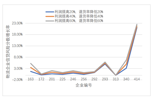
From the logistics enterprise lending risk re-evaluation results, under the three scenarios, the enterprise risk score growth rates show an overall upward trend. This indicates that as profit levels increase and return rates decrease, the enterprise’s profitability strengthens, the comprehensive risk score improves, and thus the default risk relatively decreases.
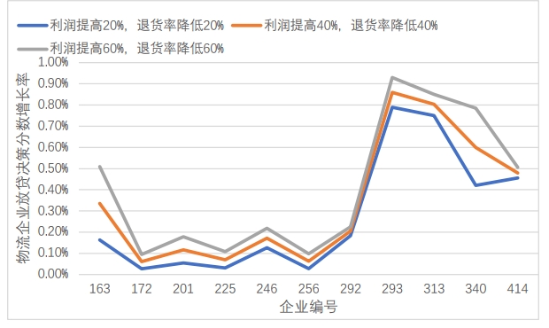
From the logistics enterprise lending decision score re-evaluation results, a similar pattern to the risk scores is also observed: the higher the enterprise’s profit margin and profit growth rate and the lower the return rate, the more significant the growth in its lending decision score. This indicates that sudden factors do not necessarily only bring negative impacts. For industries like logistics that benefit from special environments, enterprise comprehensive strength may even strengthen.
Based on this result, when facing similar scenarios, banks can consider adopting more proactive credit adjustment strategies for related industries, such as appropriately lowering access thresholds, reducing loan annual interest rates, or increasing credit quotas within controllable risk limits. This not only helps control customer churn rates but also enhances the bank’s own returns during periods of industry prosperity improvement.
5.3 Dynamic Adjustment Mechanism
The significance of stress testing is not only to provide a one-time scenario conclusion but more importantly to form a dynamic adjustment mechanism. When significant changes occur in the external environment, banks can based on industry attributes and enterprise indicator changes, timely recalculate lending capacity evaluation values and risk evaluation values, and simultaneously modify interest rates, quotas, and access conditions.
In other words, what Problem 3 provides is not a fixed answer but a strategy update framework that can be repeatedly used under sudden scenarios: first identify shock factors, then set scenario assumptions, subsequently re-evaluate enterprise scores, and finally adjust credit strategies. This can significantly enhance the model’s robustness and practical applicability in complex environments.
6. Conclusion
This article constructs a complete quantitative analysis framework for SME credit decisions around the core issues of enterprise evaluation, risk pricing, and strategy optimization. In Problem 1, the credit decision is decomposed into two levels: “whether to lend” and “how to lend.” The former computes the enterprise lending capacity evaluation value $LEND_i$ through the lending decision model to complete the loan approval judgment; the latter computes the comprehensive risk evaluation value $RISK_i$ through the credit risk evaluation model to further determine loan interest rates and credit quotas. In this way, the originally somewhat vague credit decision process is decomposed into a two-stage modeling process with clear structure, explicit logic, and strong interpretability.
In specific solution approaches, this article comprehensively uses the analytic hierarchy process, TOPSIS method, fuzzy comprehensive evaluation, and time-weighted aggregation. Among them, AHP is mainly responsible for determining the weights of the criterion layer, indicator layer, and time dimension; TOPSIS is used for multi-attribute comprehensive scoring of enterprise strength; fuzzy comprehensive evaluation is used to handle qualitatively strong indicators such as supply-demand relationship stability, enabling them to be incorporated into a unified evaluation system; and time weights are used to complete cross-year information integration. Based on this combined method, the model not only reflects the enterprise’s current business performance but also takes into account the importance differences of information across different years, thereby improving the stability of credit judgments.
In Problem 2, to address the missing “credit rating” and “default history” fields for enterprises without historical credit records, this article introduces a decision tree model to complete credit label supplementation, and then the supplemented samples are re-connected to the credit framework of Problem 1 for continued calculation. This achieves a closed-loop process of “first supplementing data, then making decisions,” enabling enterprises that could not directly enter the credit model to also complete loan approval, interest rate allocation, and quota division under a unified evaluation standard.
In Problem 3, this article further introduces the stress testing method, taking the logistics industry as an example to simulate the impact of sudden factors on enterprise business indicators and credit strategies. By setting multiple scenarios of profit improvement and return rate decline, the lending decision scores and risk evaluation scores are recalculated, and the credit strategy is dynamically adjusted based on the results. This shows that the model is not only suitable for static historical data analysis but also has certain scenario expansion capabilities, which can be used by banks for strategy revision and risk response in complex business environments.
Overall, the model established in this article possesses strong interpretability, operability, and expandability, and can well support banks in making more systematic and quantitative credit decisions for small and medium enterprises under fixed total credit constraints.
7. Model Evaluation and Reflection
7.1 Advantages of Method Combination
From the perspective of method combination, the greatest advantage of this article is the construction of a comprehensive evaluation system with clear hierarchy and tight cohesion. The lending decision model is responsible for judging whether an enterprise has basic lending eligibility, while the credit risk model is responsible for further completing interest rate and quota allocation after approval. The clear division of labor between the two not only avoids a single scoring model from bearing too many tasks simultaneously but also makes the model structure more aligned with the actual bank credit process.
At the indicator solution level, the combination of AHP, TOPSIS, and fuzzy comprehensive evaluation has strong complementarity. AHP can systematize experience-based judgments and is suitable for handling weight allocation in multi-layer indicator systems; TOPSIS can give relatively stable comprehensive ranking results among multiple quantitative indicators; and fuzzy comprehensive evaluation compensates for the deficiency that qualitative indicators are difficult to directly measure, enabling indicators such as supply-demand relationship stability to be incorporated into a unified evaluation system. After combining these three methods, the model retains its mathematical structure while enhancing the realism of its interpretations.
From the perspective of application expandability, this article does not limit the model to the scenario of “enterprises with historical credit records” but further uses decision trees to complete label prediction, enabling enterprises without historical credit to also be incorporated into the same analysis framework. Additionally, in Problem 3, the stress testing method is introduced to extend the static credit model to sudden scenario analysis. This indicates that the modeling framework in this article is not a one-time conclusion tool but a strategic analysis framework that can be continuously expanded based on data conditions and business scenarios.
7.2 Model Limitations
Although the model overall has good interpretability and operability, there are still several limitations. First, some judgment matrices in AHP rely on manually assigned values based on experience. Different researchers may have different understandings of indicator importance, so the weight results carry a certain degree of subjectivity. Although this article conducts consistency checks, passing the consistency check does not mean the weights are necessarily optimal; it only indicates that the judgment matrix is basically self-consistent internally.
Second, although the decision tree part solves the problem of missing credit labels for Attachment 2 enterprises, its training samples come only from the 123 enterprises in Attachment 1, with a relatively limited sample size, and the feature dimensions used for prediction are also relatively simplified. Therefore, the model’s generalization ability on out-of-sample enterprises is still limited, and the predicted “credit rating” and “default history” are more suitable as approximate labels rather than completely replacing real long-term credit history.
Third, most of the indicators constructed in this article still heavily rely on historical transaction invoice data, such as profit margins, profit growth rates, return rates, and stable customer proportions. This means the model is relatively friendly to enterprises with existing business records but its recognition ability is limited for enterprises with sparse transaction data, in early growth stages, or with incomplete financial records.
Finally, the stress testing in Problem 3 is still based on scenario assumptions. Whether choosing the logistics industry or setting specific proportions for profit improvement and return rate decline, there is a certain degree of empirical judgment. Sudden shocks in real environments are often more complex, and there are also significant heterogeneities among industries. Therefore, the conclusions in this part are more suitable as strategic simulation references rather than precise prediction results.
7.3 Improvement Directions
If the model effect is to be further improved in the future, optimization can be continued from the following directions. First, in the label prediction part, ensemble learning models such as random forests, XGBoost, or LightGBM can be introduced to replace single decision trees, thereby improving the stability and generalization of “credit rating” and “default history” predictions. Especially as the sample size gradually expands, ensemble models usually achieve better classification performance.
Second, in the construction of the indicator system, more external information can be appropriately introduced, such as enterprise financial statements, industry prosperity, upstream-downstream concentration, operating region, public opinion risk, and legal person profiles, thereby reducing the model’s dependence on single-source invoice data. This not only improves the completeness of enterprise portraits but also helps enhance the model’s adaptability to different types of enterprises.
Third, at the credit strategy level, differentiated modeling can be further advanced for different industries, customer segments, and life cycles. For example, more tailored indicator systems and risk mapping rules can be established for manufacturing, logistics, and trading industries, rather than completely using a unified model caliber. This can further improve the refinement and business landing effect of credit strategies.
Fourth, in the stress testing part, the expansion from a single-industry example to multi-industry, multi-shock factor joint testing, combined with a dynamic monitoring mechanism for periodic reassessment, can be conducted. In this way, the model is not just a static analysis tool but can gradually evolve into a dynamic credit decision system for actual risk management.